
$-*."5&$)"/(&"%"15"5*0/'034."--)0-%&3
'"3.&34*/4065)"'3*$"
70-6.&1"35"/*.1-&.&/5"5*0/"/%4611035(6*%&
'*&-%$3011*/("/%-*7&450$,*/5&(3"5*0/13"$5*$&4
77

Climate Change Adaptation for
Smallholder Farmers in
South Africa
Volume 2 Part 4: An implementation
and support guide: Field cropping
and livestock integration practices
E Kruger, MC Dlamini, T Mathebula, P Ngcobo, BT Maimela & L Sisitka
Report to the
Water Research Commission
by
Mahlathini Development Foundation
WRC Report No. TT 841/5/20
February 2021

ii
Obtainable from
Water Research Commission
Private Bag X03
Gezina, 0031
orders@wrc.org.za or download from www.wrc.org.za or www.mahlathini.org
The publication of this report emanates from a project entitledCollaborative knowledge creation and
mediation strategies for the dissemination of Water and Soil Conservation practices and Climate Smart
Agriculture in smallholder farming systems. (WRC Project No.K5/2719/4)
This report forms part of a series of 9 reports. The reports are:
Volume 1: Climate Change Adaptation for smallholder farmers in South Africa. An implementation
and decision support guide. Summary report. (WRC Report No. TT 841/1/20)
Volume 2 Part 1: Community Climate Change Adaptation facilitation: A manual for facilitation of
Climate Resilient Agriculture for smallholder farmers. (WRC Report No. TT 841/2/20)
Volume 2 Part 2: Climate Resilient Agriculture. An implementation and support guide: Intensive
homestead food production practices. (WRC Report No. TT 841/3/20)
Volume 2 Part 3: Climate Resilient Agriculture. An implementation and support guide: Local, group-
based access to water for household food production. (WRC Report No. TT 841/4/20)
Volume 2 Part 4: Climate Resilient Agriculture. An implementation and support guide: Field cropping
and livestock integration practices. (WRC Report No. TT 841/5/20)
Volume 2 Part 5: Climate Resilient Agriculture learning materials for smallholder farmers in English.
(WRC Report No. TT 841/6/20)
Volume 2 Part 6: Climate Resilient Agriculture learning materials for smallholder farmers in isiXhosa.
(WRC Report No. TT 841/7/20)
Volume 2 Part 7: Climate Resilient Agriculture learning materials for smallholder farmers in isiZulu.
(WRC Report No. TT 841/8/20)
Volume 2 Part 8: Climate Resilient Agriculture learning materials for smallholder farmers in Sepedi.
(WRC Report No. TT 841/9/20)
DISCLAIMER
This report has been reviewed by the Water Research Commission (WRC) and approved for
publication. Approval does not signify that the contents necessarily reflect the views and policies of
the WRC, nor does mention of trade names or commercial productsconstitute endorsement or
recommendation for use.
ISBN 978-0-6392-0231-0
Printed in the Republic of South Africa
© WATER RESEARCH COMMISSION

iii
ACKNOWLEDGEMENTS
The following individuals and organisations deserve acknowledgement for their invaluable
contributions and support to this project:
Chris Stimie (Rural Integrated Engineering – RIEng)
Dr Brigid Letty and Jon McCosh (Institute of Natural Resources – INR)
Nqe Dlamini (StratAct)
Catherine van den Hoof (Researcher)
Dr Sharon Pollard, Ancois de Villiers, Bigboy Mkabela and Derick du Toit (Association for Water and
Rural Development)
Hendrik Smith (GrainSA)
Marna de Lange (Socio-Technical Interfacing)
Matthew Evans (Web developer)
MDF interns and students: Khethiwe Mthethwa, Samukhelisiwe Mkhize, Sylvester Selala, Palesa
Motaung and Sanelise Tafa
MDF board members: Timothy Houghton and Desiree Manicom
PROJECT FUNDED BY
REFERENCE GROUP MEMBERS
Prof S Mpandeli Water Research Commission
Dr S Hlophe-Ginindza Water Research Commission
Dr L NhamoWater Research Commission
Dr O CrespoUniversity of Cape Town
Dr A Manson KZN Department of Agriculture and Rural Development
Prof S WalkerAgricultural Research Council
Prof CJ RautenbachPreviously of WeatherSA
COLLABORATING ORGANISATIONS
https://inr.org.za/https://award.org.za/https://amanziforfood.co.za/
https://foodtunnel.co.za/http://www.rieng.co.za/

iv
ABBREVIATIONS AND ACRONYMS
Al Aluminium
C Carbon
Ca Calcium
CA Conservation Agriculture
CC Climate change
CCA Climate change adaptation
CRA Climate resilient agriculture
CO2 Carbon dioxide
ET Evapotranspiration
Fe Iron
K Potassium
MDF Mahlathini Development Foundation
N Nitrogen
NH4 Ammonium
NO3 Nitrate
OM Organicmatter
P Phosphate
SCC Summer cover crops
SH Soil health
SOC Soil organic carbon
SOM Soil organic matter
WP Waterproductivity

v
TABLE OF CONTENTS
ACKNOWLEDGEMENTS .......................................................................................................................iii
PROJECT FUNDED BY..........................................................................................................................iii
REFERENCE GROUP MEMBERS ........................................................................................................iii
COLLABORATING ORGANISATIONS ..................................................................................................iii
ABBREVIATIONS AND ACRONYMS ................................................................................................ iv
TABLE OF CONTENTS .......................................................................................................................... v
1BACKGROUND AND INTRODUCTION .......................................................................................... 1
1.1CLIMATE RESILIENT FIELD CROPPING PRACTICES ........................................................ 1
1.2SITES AND PARTICIPANTS .................................................................................................. 1
1.2.1INNOVATION SYSTEM PROCESS ................................................................................... 2
1.3CURRENT STATUS OF FIELD CROPPING .......................................................................... 3
1.3.1LIMPOPO ............................................................................................................................ 3
1.3.2KWAZULU-NATAL .............................................................................................................. 4
1.3.3FARMERS COMMENTS REGARDING CLIMATE CHANGE IMPACTS ON FIELD
CROPPING......................................................................................................................... 4
2CRA IMPLEMENTATION: FIELD CROPPING................................................................................ 6
2.1RESULTS: LIMPOPO ............................................................................................................. 6
2.1.12017-2018 ........................................................................................................................... 6
2.1.22018-2019 ........................................................................................................................... 7
2.1.32019-2020 ........................................................................................................................... 9
2.2RESULTS: KWAZULU-NATAL (KZN) .................................................................................. 12
2.2.1RAINFALL AND RUNOFF SUMMARIES FOR 2019-2020 SEASON .............................. 12
2.2.2SOIL HEALTH CONSIDERATIONS ................................................................................. 18
2.2.3YIELD CONSIDERATIONS .............................................................................................. 26
2.2.4BULK DENSITY ................................................................................................................ 28
2.2.5WATER PRODUCTIVITY ................................................................................................. 30
2.2.6EXAMPLES OF FARMER-LEVEL EXPERIMENTATION IN BERGVILLE ....................... 33
2.3LIVESTOCK INTEGRATION ................................................................................................ 34
2.3.1COVER CROP MIXES ...................................................................................................... 34
2.3.2WINTER FODDER SUPPLEMENTATION EXPERIMENTATION.................................... 34
2.3.3STRIP CROPPING WITH PERENNIAL FODDER SPECIES ........................................... 36
3BEST PRACTISE OPTIONS IN LEARNING METHODOLOGY.................................................... 39
3.1LEARNING METHODOLOGY .............................................................................................. 39
3.2PRACTICAL DEMONSTRATIONS....................................................................................... 39
3.2.1NO-TILL PLANTERS ........................................................................................................ 41
3.2.2FACILITATORS’ REFLECTIONS ON THE CA LEARNING PROCESS .......................... 42
4REFERENCES .............................................................................................................................. 43

1
1 BACKGROUND AND INTRODUCTION
1.1 CLIMATE RESILIENT FIELD CROPPING PRACTICES
CRA field cropping practices include a suite of practices that focus on soil and water conservation and
soil health alongside the conventional soil fertility and soil structure considerations. Attention is also
given to crop diversification, crop types and varieties that are more suitable to the changing conditions.
Different planting dates are considered, as are options for extending the growing season. Livestock
integration is considered to be an important aspect of the process and in the development of climate
resilient local value chains.
Sustainable and regenerative agricultural practices such as conservation agriculture (CA), that
conserve and increase soil organic carbon (SOC) and improve soil health, are increasingly promoted
in Southern Africa as an alternative to conventional farming systems (Smith et al., 2017). CA depends
on the simultaneous implementation of three linked principles: (1) continuous zero or minimal soil
disturbance, (2) permanent organic soil cover, and (3) crop diversification, specifically with the inclusion
of legumes and/or cover crops (FAO, 2013).
Complementary practices supporting CA implementation in smallholder farming systems include
appropriate nutrient management and stress-tolerant crop varieties, increased efficiency of planting and
mechanisation, integrated pest and disease and weed management, livestock integration, and enabling
political and social environments (Thierfelder et al., 2018).
To pilot these practices in different localities, participants organised into learning groups, considered
local adaptive measures and included practices promoted through the smallholder decision support
system that were appropriate to their own systems. Generally, these practices are piloted through the
innovation system development process and local farmer-level experimentation. Farmers deepen and
expand their experimentation options over a three- to four-year period of learning and try out different
options. This is crucial in knowledge-intensive farming systems.
Practices that were piloted by the learning groups included: CA, intercropping, crop rotation, micro-
dosing with fertilizer, drought tolerant crops, integrated weed and pest management and livestock
integration through production of cover crops appropriate for livestock fodder as well as production of
hay and winter supplementation. Soil and water conservation practices included planting on contour,
stone lines, check dams and planting agroforestry species such as Pigeon pea and Sesbania sesban.
1.2 SITES AND PARTICIPANTS
Sites were chosen to be representative of different agroecological conditions within South Africa.
Province Area VillagePractices Number of participants (No. in
brackets indicate those who
g
ot a harvest
)
2017/18 2018/19 2019/20
Limpopo Mametja Sedawa,
Turkey,
Willows,
Botshabelo,
Santen
g
CA, intercropping, drought tolerant crops,
livestock integration, stone lines, check dams
and planting agroforestry species
28 (0) 45 (15) 35 (10)
KZN Bergville Ezibomvini,
Stulwane,
Eqeleni,
Ndunwane
CA, intercropping, crop rotation, micro-dosing
with fertilizer, drought tolerant crops,
integrated weed and pest management and
livestock inte
g
ration
95 (76) 78 (59) 94 (80)
KZN SKZN Madzikane,
Ofafa, Spring
Valley
CA, intercropping, crop rotation, micro-dosing
with fertilizer, drought tolerant crops,
integrated weed and pest management and
livestock inte
g
ration
30 (21) 40 (29) 60 (51)
KZN Midlands Gobizembe,
Mayizekanye,
Ozwathini
CA, intercropping, micro-dosing with fertilizer,
drought tolerant crops, integrated weed and
pest mana
g
ement and livestock inte
g
ration
32 (26) 62 (54) 122
(91)
EC ??? Xumbu CA, deep ripping, intercropping, crop
diversification and short furrow irri
g
ation
8 (0) 15 (0) 6 (0)

2
1
1.2.1
Innovation system process
The process starts with an introductory workshop with each of the learning groups, to introduce the
concepts and practices and discuss inclusion of these into their present farming systems, followed by
practical demonstrations and setting up the farmer-level experimentation trial plots.
Interested individuals in a local area or village come together to form a learning group. Several farmers
in that group then volunteer to undertake on-farm experimentation, which creates an environment where
the whole group learns throughout the season through observations and reflections on the trials’
implementation and results. They compare various treatments with their standard practices, which are
planted as control plots.
For the field cropping piloting process, CA formed the backbone of the experimentation process, around
which other practices were built and included. The CA principles best embody the adaptive processes
required, with outcomes that include improved soil organic matter, soil aggregation and soil health as
well as improved water holding capacity and reduced runoff.
A detailed description of the community-level process for introduction and experimentation for CA is
provided in the text box below.

3
*Introducing organic CA options into a farming system where soil structure has been destroyed through repeated
ploughing, where there is very low fertility and soil organic matter and where weed pressure is high due to ongoing
lack of management is particularly challenging. Rehabilitation of such systems is unlikely to gain traction unless
initial remedial activities are undertaken, which should include incorporation of large amounts of organic matter,
some form of mulching and soil cover, soil and water conservation structures and soil pH amelioration through
addition of lime and/or gypsum.
This report focuses on a qualitative assessment of CA introduction in Limpopo and inclusion of several
quantitative assessments for the Bergville area in KwaZulu-Natal. In the Eastern Cape, crop failure was
experienced for all three seasons of implementation, which reduced opportunities for learning and
continued farmer-level experimentation.
1.3 CURRENT STATUS OF FIELD CROPPING
1
1.3.1
Limpopo
Dryland cropping is a common practice in the area, although it has declined dramatically with the five-
year drought in the area, compounding ongoing reduction in cropping due to low soil fertility, access to
seed and inputs, and lack of labour.
SELECTION AND COMMUNITY-LEVEL PROCESS
PRECONDITION: Farmers active in field cropping with some level of social organisation.
1. Entry into community – through word of mouth from community members (individual and group
requests), government officials, other service organisations.
2. Set up introductory meetings at community level, including authorities, to introduce CA and the
process:
3. Set up learning or interest group (20-30 people).
a. Setting up of VLSA’s (village savings and loan associations), farmer centres and joint
harvesting, storage and milling options are promoted
4. Members of learning group volunteer for farmer-led experimentation (usually 9-12 members in the first
year), while the rest of the group learns alongside them.
5. These members agree to do a CA trial alongside their control (normal way of planting).
a. Trials are usually 100 m2, 400 m2 or 1 000 m2 (small areas to reduce risk).
6. The programme provides inputs for the trial; the inputs for control and all labour are provided by the
farmer (the risk of implementing the new idea initially sits with the programme not the farmers. From
the second year the farmers pay a standard 30% subsidy towards the costs of inputs for their trials).
a. Planters and knapsack sprayers are provided to the learning group to share, manage and
maintain
7. Farmers are trained in the implementation of CA – pre-planting spraying (use of knapsack sprayers)
and field preparation, use of herbicides, layout of plots and planting in basins and rows using a range
of no-till tools (hand planters, animal drawn planters and/or two-row tractor-drawn planters). The
choice of implements depends on the scale of farming and farmers’ choices. Aspects such as top
dressing, weeding and pest control are covered during the season as well. Organic CA cropping
systems are explored in areas where participants prefer this option*.
a. As a minimum, 2-4 learning sessions per season in the learning group are held each year,
building in complexity and content. This includes one review session for the season and one
planning session to plan experimentation for the upcoming season.
8. The first-year trial layout is predetermined through the programme – to include close spacing,
intercropping and different varieties of maize (choice of traditional OPV or hybrid seed, according to
farmer preferences) and legumes (sugar beans, cowpeas).
9. From the second year, farmers start to add their own elements to the experimentation depending on
their learning, questions and preferences. Cover crops (both summer and winter) and crop rotation
options are introduced.
10. Researcher-managed “trials” are also set up at individual homesteads to work alongside the more
enthusiastic and committed participants and to explore issues such as soil health, carbon
sequestration, soil fertility, water productivity, moisture retention, runoff and specific aspects of the CA
system, such as seeding and seeding rates of cover crops, etc.
11. Each season farmers days are organised in each area, jointly with the learning groups. CA forums and
innovation platforms are promoted where all stakeholders in a region join these forums to share,
discuss and plan together. This includes role players such as DARD, Social Development, LandCare,
Local and District Municipalities, Agribusiness service providers and NGOs

4
Learning group participants are very keen to re-initiate or continue field cropping aspects of their
farming. Presently most participants undertake this activity within their extended homestead plots, with
only a small proportion of participants having access to larger fields and or supplementary irrigation
options.
With the shift in weather patterns and climate variability, (increased heat, late onset and unpredictability
of rains) the field cropping practice in the area has already shifted; surprisingly away from the more
drought tolerant crops such as millet and sorghum, towards maize with supplementary irrigation. This
is due to much greater predation of the millet and sorghum by birds (in particular), but also monkeys
and wildlife than was experienced in the past. Farmers are aware of bird-resistant sorghum varieties
but have not been able to access seed. They also practice protection of the seed heads with netting as
an adaptive strategy. Planting of traditional leguminous crops such as ground nuts, jugo beans
(bambara ground nut) and cowpeas is still popular, as is planting of pigeon pea and moringa. Other
field crops include pumpkin and watermelon. Some farmers have started experimentation with different
planting calendars.
1
1.3.2
KwaZulu-Natal
In the Bergville area, communities still practice field cropping primarily for food security and rely on their
maize harvests for food. Dryland cropping, focusing almost exclusively on maize and extensive livestock
management are the main activities. There has been a sharp reduction in field cropping over the last
15 years, given stress factors such as uncontrolled livestock, increased poverty, difficulties in accessing
tractors, expensive inputs and climate change.
In the Midlands and SKZN regions, with higher rainfalls and easier access to markets in urban centres,
the focus has been more on the production of green mealies and livestock feed (yellow maize). These
farmers also focus on other field crops such as amadumbe (taro), pumpkin, beans and sweet potato,
and produce a range of vegetables. Here a much larger proportion of the fields are fenced, compared
to Bergville, as livestock invasions in these more densely populated areas is a large risk factor with
cropping.
In more general terms, field cropping in KZN is hampered by soil acidity, lack of appropriate nutrient
and weed management and continued monocropping of maize. Mazie yields are generally very low and
average t/ha.
1.3.3
Farmers comments regardingClimate Change impacts on field cropping
x“Lack of rainfall and changes in rainfall patterns have been a major challenge with regard to
both field cropping and homestead gardening.”
x“Pest outbreaks which are associated with extreme heat have been worse, especially on
maize.”
x“Repeated crop failure has meant that we no longer have seed to plant our field crops.”
x“When it does rain there is now a lot more erosion, because the soil is not covered.”
Farmers comments regardingCA implementation in the context of CC
x“The CA process has brought the community together and is helping farmers to groom each
other to improve our farming.”
x“Better yields have been observed, specifically for maize, as well as better weed knowledge
and management skills.”
x“Maize planted after Lablab can be highly productive. However, lablab and cover crops are
inedible and they are very attractive to livestock, hence most farmers are resistant to
diversifying, they only use maize.”
x“Those who obtain higher yields are the hard workers, as weeds are likely to be a big problem
if weeding is not done carefully and on time.”
x“Soil management has improved under CA, both soil fertility and much reduced erosion and
yields have improved dramatically.”

5
x“CA is cost effective and cheaper than conventional tillage as tractors need not be hired and
fertilizer and other inputs are used sparingly.”
x“Most of the participants have decreased fertilizer use and increased use of manure on their
fields. The results are still good.”
x“Having savings groups has helped a lot in terms of buying inputs.”
6
2 CRA IMPLEMENTATION:FIELD CROPPING
During each season, a set of CA experiments is decided upon, followed by demonstration workshops
at farm level, implementation by all volunteers and ongoing monitoring. Observations are recorded and
discussed with the learning groups in their seasonal review of their experimentation process, to allow
for planning of the next experimentation cycle.
For the results section below, the Limpopo CA implementation activities have been divided into specific
experiments, with aims, process and observations recorded for each.
2.1 RESULTS:LIMPOPO
2
2.1.1
2017-2018
AIM: Introduction of CA principles and close spacing, intercropping with legumes, planting bird-resistant
sorghum and CA planters.
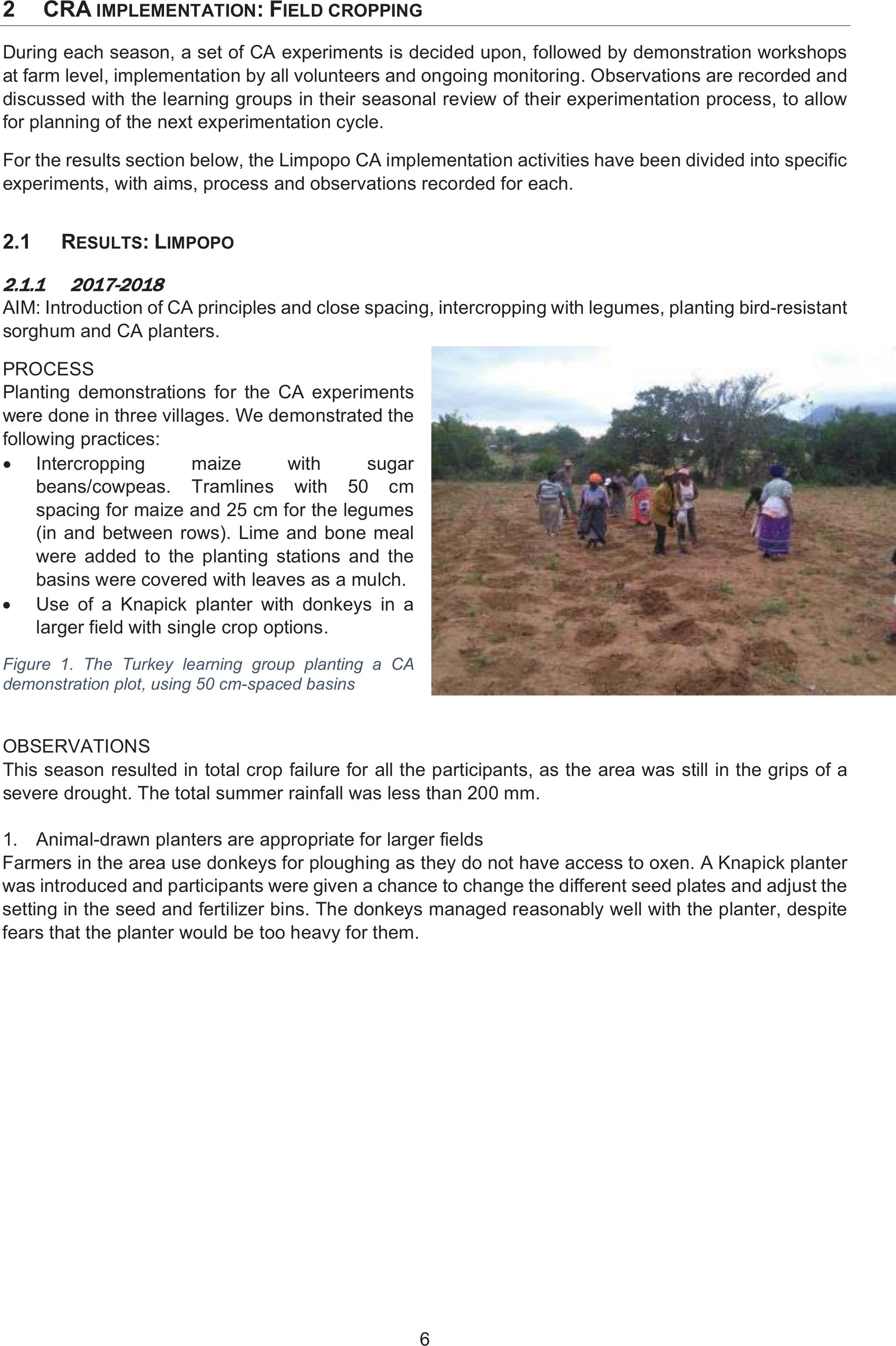
PROCESS
Planting demonstrations for the CA experiments
were done in three villages. We demonstrated the
following practices:
xIntercropping maize with sugar
beans/cowpeas. Tramlines with 50 cm
spacing for maize and 25 cm for the legumes
(in and between rows). Lime and bone meal
were added to the planting stations and the
basins were covered with leaves as a mulch.
xUse of a Knapick planter with donkeys in a
larger field with single crop options.
Figure 1. The Turkey learning group planting a CA
demonstration plot, using 50 cm-spaced basins
OBSERVATIONS
This season resulted in total crop failure for all the participants, as the area was still in the grips of a
severe drought. The total summer rainfall was less than 200 mm.
1. Animal-drawn planters are appropriate for larger fields
Farmers in the area use donkeys for ploughing as they do not have access to oxen. A Knapick planter
was introduced and participants were given a chance to change the different seed plates and adjust the
setting in the seed and fertilizer bins. The donkeys managed reasonably well with the planter, despite
fears that the planter would be too heavy for them.

7
Figure 2. Left: Introducing the Knapick planter to the learning group and demonstrating the changing of seed plates.
Right: The oxen-drawn planter has been hitched to a team of donkeys for planting.
Some of the challenges were:
xNot being able to control the donkeys (they could not plant in a straight line, meaning it was
hard to maintain a consistent inter-row spacing) – this could have been because the donkeys
were not well trained.
xLearning to change the planting discs requires hands-on practice for each participant, which
took a lot of time.
xThe soils at planting were very wet and clayey (a sandy clay), which meant that the planting
tines kept getting blocked. This showed the group that planting with this planter would need to
be undertaken once the soil has drained.
xTransporting the planter from one site to the other was a problem, as it requires a long-wheel-
base LDV.
Despite the above-mentioned challenges, participants liked the planter and felt it would be very useful
to have one in each of the villages.
2
2.1.2
2018-2019
AIM: Review of CA principles and practice to date and close spacing and intercropping with legumes.
For this season, CA principles were reviewed, and experimentation focused on close spacing and
intercropping as these aspects were not well internalised in the first cropping season.
PROCESS
Planting demonstrations for the CA experiments were done in three villages. We demonstrated the
following practices:
xIntercropping maize with sugar beans/cowpeas.
xTramlines with 50 cm spacing for maize and 25 cm for the legumes (in and between rows).
OBSERVATIONS
1. Close spacing and intercropping improves crop stand and growth.
Farmers noticed the difference between their local system and the CA experiments. First, they noticed
that the narrow spacing of crops in the CA system worked a lot better than the preferred wider spacing
in the area. They worked on the understanding that the wider spacing reduces water stress, as does
monocropping, but found that the intercropping and close spacing increased the potential of survival of
their crops considerably. They realised that the cover provided by the closely spaced grain-legume
intercrop improves water holding and reduces the effect of extreme heat.
8
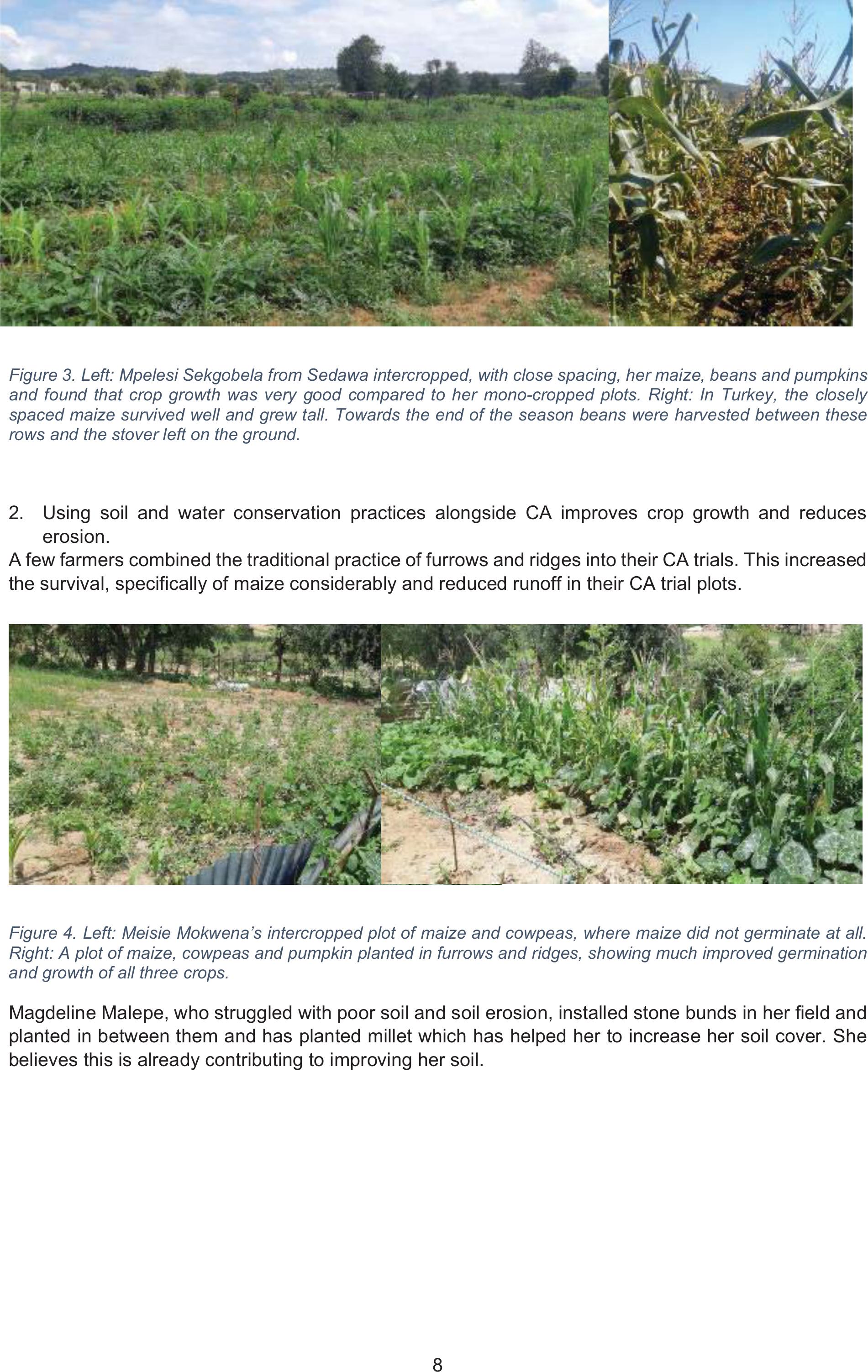
Figure 3. Left: Mpelesi Sekgobela from Sedawa intercropped, with close spacing, her maize, beans and pumpkins
and found that crop growth was very good compared to her mono-cropped plots. Right: In Turkey, the closely
spaced maize survived well and grew tall. Towards the end of the season beans were harvested between these
rows and the stover left on the ground.
2. Using soil and water conservation practices alongside CA improves crop growth and reduces
erosion.
A few farmers combined the traditional practice of furrows and ridges into their CA trials. This increased
the survival, specifically of maize considerably and reduced runoff in their CA trial plots.
Figure 4. Left: Meisie Mokwena’s intercropped plot of maize and cowpeas, where maize did not germinate at all.
Right: A plot of maize, cowpeas and pumpkin planted in furrows and ridges, showing much improved germination
and growth of all three crops.
Magdeline Malepe, who struggled with poor soil and soil erosion, installed stone bunds in her field and
planted in between them and has planted millet which has helped her to increase her soil cover. She
believes this is already contributing to improving her soil.

9
Figure 5. Magdalene Malepe’s planted field, showing the stone lines
above and below the four rows of maize in the picture
Other observations made by farmers for this season of
experimentation included the following:
xFarmers observed that soil in the CA plot holds moisture
longer than their traditionally planted plots.
xFarmers observed less competition between the crops in
their CA plots compared to their traditional planting
method.
xMr Mogofe: “I tried what we were taught last year and I
realised that the moisture lasts longer in the CA plot
compared to the normal plot.”
xSarah Madire added that with addition of manure and
leaving soil cover even the colour of the soil was starting
to change: “this could indicate that with time, yes, this can
help improve our soil.”
xSome participants felt that they could see some
improvement in the CA trials from last season, but not that
much. Some participants, however, felt that CA was a
long-term strategy and it will take a while before they see some of the benefits of CA (e.g.
improvement in soil structure).
2
2.1.3
2019-2020
AIM: Review of CA principles and practice to date and conscious inclusion of summer cover crops and
Dolichos (Lablab) beans into the cropping system.
Farmer-level experiments were introduced – differing depending on whether participants had already
planted portions of their fields and on the cover crops they were interested in trying. Sunflower is known
as a heat- and drought-resistant crop but is not grown much anymore as participants are no longer
keeping poultry (due to lack of water). They asked about potential markets. Dolichos is popular as both
the leaves and seed can be eaten.
PROCESS
Planting demonstrations for the CA experiments were done in four villages. We demonstrated the
following practices:
xPlanting maize with a summer cover crop mix (Babala/millet, sunflower and Sun hemp), or
individual cover crops such as sunflowers. Four rows of maize were planted in basins 50 cm
apart and four rows of cover crops planted in furrows 25 cm apart at a rate of 10 kg/ha. Cover
crops were relay planted into the maize, three to four weeks after planting maize, to reduce
moisture competition between the crops.
xIntercropping maize with sugar beans/cowpeas. Tramlines with
50 cm spacing for maize and 25 cm for the legumes (in and
between rows).
xDolichos (Lablab beans) were planted along fence lines
according to the local practice. Participants did not want to plant
Dolichos as an intercrop, fearing competition with other crops.
xBales of grass were used to mulch portions of the CA trials, to
test the effect on weed suppression and moisture retention.
xHand weeding was undertaken during the season and weeds
were left on the soil surface as a mulch.
Figure 6. Right: Mulching a portion of the CA trial plot in
Turkey

10
OBSERVATIONS
Only ten of the 35 participants in the CA experimentation cycle managed to grow crops that were
harvestable. For most of the participants, germination was low, and crops died back soon after
germination. Weather conditions were unconducive, with intense heat and low rainfall between
December 2019 and January 2020. In addition, lack of soil fertility and soil organic matter was a major
limiting factor.
1. Summer cover crops (Sun hemp, sunflower and millet) survived where maize and legumes
such as beans and cowpeas died back due to heat and drought stress.
Magdalene Malepe: “Sun hemp has grown very well and it is a good crop for provision of fodder for
goats. Intercropping with Sun hemp works much better because I have seen an improvement in my
soil.”
Figure 7. Left: Magdalene’s Sun hemp, intercropped with maize growing very well. The maize, however, is showing
strong signs of heat and water stress and most has already died back. Right: Maize roots are stunted and growing
horizontally, indicative of a highly compacted soil and a shallow plough pan typical of plots where hand hoes have
been used for tillage for many years.
Figure 8. In Turkey, all
Sarah Madire’s summer
cover crops survived well
(Babala, sunflower and
Sun hemp), along with a
few straggly maize plants
2. Cowpeas can still do well under difficult conditions if adequate mulching is provided.
Magdalene Malepe is aware that her soil is not very fertile and has issues. In this regard, she decided
to do a small experiment with lime by herself – she added lime to a section of her plot where she planted
cowpeas and another small area with cowpeas without lime. She also mulched these plots. She saw
that the cowpeas that received lime and mulch grew much better and were a good dark green colour
compared to those without lime or mulch, which showed purpling on the leaves.

11
Figure 9. Right: Cowpeas growing well, with
added lime and mulch
Note: From soil fertility samples analysed for
these participants, it was determined that lime is
not required in this system and pH of the soil
averages around pH 7,5.
3. Adding organic matter to the
soil for improved soil fertility
allows maize to grow where it
otherwise would not – where
conditions are hot and dry.
Meisie Mokwena from Sedawa makes
piles of organic matter in her field at
the end of the season to improve
her soil fertility and makes and
adds compost to her soil.
Figure 10. Meisie’s maize, gourd and
moringa intercropped plot, planted in
soil with organic matter added. Her
maize has thrived, while that of her
neighbours, who do not add organic
matter, died back.
4. Supplementary irrigation
can assist in survival of crops, specifically maize.
Angelina Thekwane from Turkey intercropped maize with Sun hemp and provided supplementary
irrigation, using municipal water. This provided for good growth of both crops, although the maize lacked
nutrients (as she plants without adding anything to the soil) and maize roots were shallow, indicative of
soil compaction.
Figure 11. Left:
Angelina’s maize and
Sun hemp intercrop
growing remarkably
well. Centre: Angelina
holding a maize cob.
Right: A root ball of
one of the maize
plants. This indicates
compacted, low fertility
soil.
5. Traditional legumes that are heat- and drought-tolerant such as groundnuts and jugo beans are
a good alternative to maize.

12
Some participants decided against planting maize, given the bad track record for this crop over the last
few years. One such participant is Mmatshego Shaai from Turkey. She planted only legumes –
groundnuts and jugo beans, for a second season in a row. She found these crops survived better and
provided for better soil moisture due to their canopy, as well as reduced erosion in her plot.
Figure 12. Mmatshego
Shaai’s field planted to
ground nuts and jugo
beans, which she sells
in the community.
Silence Malapane in
Willows followed the
same practice. He
planted these
legumes in basins
and in ridges and
furrows. He felt that
compacted,
uncovered soil is a problem under the present conditions. This can be considered a local adaptation
and is important to note.
2.2 RESULTS:KWAZULU-NATAL (KZN)
In KZN, co-funding from the Maize Trust to implement a smallholder farmer innovation programme in
CA has allowed for more intensive farmer-level experimentation and quantitative assessments of the
results. The CA implementation has been undertaken for a longer period (4-7 years), for the five villages
(Stulwane, Eqeleni, Ezibomvini, Ndunwane and Mhlwazini), prioritised for this research process. This
has allowed us to assess some of the longer-term impacts of CA. The results presented are primarily
for the most recent cropping seasons (2019/20).
Results for the quantitative assessments undertaken (rainfall, runoff, soil fertility, soil health, bulk density
and water productivity) are presented below, followed by examples of the farmer-level experimentation
for a selection of participants.
2
2.2.1
Rainfall and runoff summaries for 2019-2020 season
2.2.1.1Introduction
In general, the average annual rainfall for the Drakensberg region ranges between 750 mm and 1 350
mm. The actual amount of rainfall has not varied much over time (besides a potential 20-year
periodicity), even for long term studies over 50 years, but the monthly variability has been increasing
quite dramatically (Nel, 2009).
Rainfall variability relates to the amount of annual rainfall as well as its seasonal distribution. This
periodicity affects the potential surface runoff, as well as subsurface and basal flows in a catchment.
To illustrate this, the following two figures indicate the monthly rainfall averages in the 2016/17 and
2019/20 seasons; indicating a shift to late onset of summer rains and increased late season rainfall
between these two seasons.

13
Figure 13. Monthly rainfall averages (mm) for Ezibomvini (2016/17)
Figure 14. Monthly rainfall averages (mm) for Ezibomvini (2019/20)
These seasonal rainfall differences have implications both for runoff and crop performance.
Runoff (stormflow or surface runoff of water) is generated by rainstorms and its occurrence and quantity
are dependent on the characteristics of the rainfall event, i.e. intensity, duration and distribution
(Schulze, 2011). There are, in addition, other important factors which influence the runoff-generating
process. These factors include the infiltration capacity of the soil, the soil moisture content when the
rainfall event occurred, the soil type, presence of capping/crusting, and slope.
In addition, the presence of above-ground vegetation intercepts some of the rainfall and reduces
raindrop impact and thus crusting of the soil. Vegetation also has a significant effect on the infiltration
capacity of the soil. The root system and organic matter in the soil increase the soil porosity thus
allowing more water to infiltrate. Vegetation also retards the surface flow, particularly on gentle slopes,
giving the water more time to infiltrate and to evaporate. Thus, vegetation reduces runoff substantially,
compared to bare ground (Critchley & Siegert, 1991).
For the purposes of comparing the effect of Conservation Agriculture on runoff in the context of an
agricultural cropping field, only surface runoff has been considered.
Runoff plots are used to measure surface runoff as well as erosion through removal of sediment under
controlled conditions. In this instance, runoff microplots, as designed previously by UKZN researchers,
(Mutema, et al., 2017) have been used.
Runoff microplots consist of galvanised metal sheeting frames 1 m by 1 m, inserted 10 cm into the
ground and leaving another 10 cm above ground to eliminate run-on water during rain events. A spirt
level was used to keep the runoff plots levelled and the slope was considered (runoff plots were not
installed on slopes greater than 7%) when installing the runoff plots. Surface water and sediment
generated are collected in a protected gutter through openings in a downslope-side metal sheet. The
gutter is fitted with a delivery pipe connected to a reservoir (in our case, a 25 L bucket with a lid) about
1,5 m downslope. After each rainfall event, the total runoff volume (ml) from each microplot replicate
OctoberNovember DecemberJanuaryFebruaryMarchAprilMay
Rainfall mm4,375,4152,2 160,8 304,387,6134,10,0
0,0
100,0
200,0
300,0
400,0
Rainfall(mm)
Monthly Rainfall in Ezibomvini 2019-2020
SeptemberOctoberNovember DecemberJanuaryFebruaryMarchAprilMay
Monthly Rainfall2,640,3 118,4 98,710297,544518
0
50
100
150
Rainfall (mm)
Monthly Rainfall in Ezibomvini 2016-2017

14
was measured with a measuring cylinder (Dlamini, et al., 2011). Sediment was noted on occasion, but
not recorded.
Figure 15: Above left: A runoff microplot installed in a CA trial plot with maize and beans, Above Centre: Installing
a runoff microplot in a conventionally tilled plot with maize and Above Right: In-season maintenance of collection
buckets
The aims of the experiments are:
1. To ascertain differences in runoff when comparing minimal tillage to conventional tillage.
2. To ascertain differences in runoff between different cropping options between the CA trial plots.
2.2.1.2Methods and results
Runoff pans were installed for four participants across four villages in the Bergville area, for the
2019/2020 planting season: Nelisiwe Msele (Stulwane), Phumelele Hlongwane (Ezibomvini), Boniwe
Hlatshwayo (Ndunwane) and Ntombakhe Zikode (Eqeleni).
Each participant also had a rain gauge set up in her homestead. Participants took records for both
rainfall and runoff for the cropping season (usually October to April). The period, however, depends on
the start and end of the rainy season.
Below is a small illustrative table indicating the number of rainfall events recorded for each participant,
with the number of runoff events recorded in brackets alongside. The number of rainfall events recorded
need to coincide closely with the number of runoff measurements taken. It is not expected that the
number of rainfall events recorded should be the same across the villages, as it is quite common in this
mountainous region for rain to fall in one village but not another nearby, due to the increasingly localised
pattern of rainfall events.
Table 1. Outline of rainfall data recorded across four village rain gauges in Bergville (2019/20)
VillageNumber of rainfall and runoff (in brackets) measurements taken
April 2020 March 2020February 2020 January 2020
Stulwane10 (10) 3 (3) 9 (9) 4 (4)
Ezibomvini 7 (6)4 (3) 4 (4) 11 (11)
Ndunwane4 (4) 6 (6) 10 (10) 14 (14)
Eqeleni12 (6)8 (6) 10 (11)20 (0)
Record keeping in Stulwane, Ezibomvini and Ndunwane is considered reliable. In Eqeleni, in addition
to the mismatch between the number of rainfall events and runoff measurements taken, all the runoff
measurements were recorded as 0,5 L or 1 L, indicating to the team that these were mostly fabricated.

15
In this case, Mrs Zikode tasked her matriculating daughter with the record keeping, given that she is
not herself literate. The Eqeleni results will thus not be considered.
Table 2. Percentage rainfall converted to runoff for three villages in Bergville (2019/20)
Jan-April 2020 Rainfall Percentage rain converted into runoff
mm CA trial Conventional control
Stulwane 394 3,87%5,33%
Ezibomvini
(January 2020-April 2020)
(October 2019-April 2020)
819
1 122 3,63%8,89%
Ndunwane 641 0,30%0,29%
SAEON weather station at Didima
(January 2020-April 2020)
(October 2019-April 2020)
687
919
Note 1: The control plot for Boniwe Hltashwayo in Ndunwane was also a minimum tillage plot (0%-15% soil disturbance), planted
to single-cropped maize with different spacing and fertilizer application regimes to her CA trial plot.
Note 2: Conventional control plots in Stulwane and Ezibomvini consisted of tilled plots (>30% soil disturbance), planted to single-
cropped maize with different spacing and fertilizer application regimes to her CA trial plot.
Note 3: Weather station data from the Ezibomvini weather station were lost and replaced by data from a SAEON weather station
at Didima (~12 km away).
The rainfall results as recorded for the rain gauge at Ndunwane
most closely resemble the data obtained from SAEON for a
weather station at Didima (KZN Parks) – 641 mm and 687 mm
respectively. This makes sense, as the community is very close
to the edge of the national park and at a similar elevation. We
suspect the rainfall data in Stulwane to be an underestimate and
that for Ezibomvini to be an overestimate. The averaged data
across the three sites, however, closely resemble the rainfall data
from the weather station used.
Figure 16: Right: Uploading data at the Ezibomvini weather station.
From Table 2 it can be seen that the percentage runoff in the
conventional control plots in Stulwane and Ezibomvini is 1,46%
and 5,26% higher than for the average CA trial plots in these
villages. In Ndunwane, runoff in both the CA trial and control plots
was negligible.
The rainfall and runoff measurements were initiated in 2016/17 in Phumelele Hlongwane’s (Ezibomvini)
CA experimentation plots. The table below gives a summary of her runoff results for the last four
cropping seasons. She has practiced CA for six consecutive seasons.
Table 3. Comparison of percentage rainfall converted into runoff for Ezibomvini 2016/17 to 2019/20
Rainfall recorded by Phumelele Hlongwane from her rain gauge is similar to the rainfall measured by
the local weather station.
Ezibomvini Rainfall (weather
station data)
Rainfall (rain
gauge)
Percentage rain converted into
runoff
mm mm CA trial Conventional control
2016/17 526 11,7% 20,1%
2017/18 455 563 12,3% 27%
2018/19 703 675 0,95% 1,11%
2019/20 9191 122 3,6% 8,9%

16
From Table 3 it can be seen that the percentage rainfall converted into runoff depends on the season
and is not directly related to the overall amount of rain. The runoff is much more closely related to
intensity of individual rainfall events, the number of such events in a rainy season, the soil moisture at
the time of the rain, as well as bulk density of the soil, compaction and soil cover. The percentage
conversion of rainfall into runoff is consistently lower, on average by 9,5% in the CA trial plots compared
to a conventionally tilled plot. These results are similar to a study conducted in Potshini village in
Bergville (Mchunu & Chaplot, 2012) which showed that minimal tillage in a small-scale agriculture
context, even with <10% crop residue cover has the potential to significantly reduce soil and soil organic
carbon losses by water.”
Stulwane
The layout of the CA experiment/trial is a combination of ten single, intercropped or multi-cropped plots,
which are rotated annually.
Table 4. Runoff measured in different plots within Nelisiwe Msele’s experiment; Stulwane (2019/20)
Stulwane: Nelisiwe Msele (2019/2020)Rainfall
Plot 1 (L)Plot 3 (L)Plot 6 (L)Plot 8 (L) Control (L) (mm)
2018/19 M+CP M B SCC M
2019/20 LL B M M M
Jan-20 3,2 0,7 0,15 3,5 3,4 40,5
Feb-20 5,9 8,7 3,0 2,95 4,72 160
Mar-20 4,052,15 1,55 3,8 3,65 92
Apr-205,0 5,32 3,7 4,05 6,1101,5
Totals 18,15 16,87 8,4 14,3 17,87 394
Note: M+CP = maize and cowpea intercrop; M = maize single crop; B = bean single crop; SCC = summer cover crop mix of
sunflower, millet and Sun hemp; LL = Dolichos beans
Data indicate increased runoff with increased monthly rainfall, which is to be expected, and quite
significant variations in runoff between the CA trial plots monitored, even though the average runoff
across these plots is lower than the runoff on the conventionally tilled control plot.
The highest recorded runoff amounts are for February and April, with highest monthly runoff for the
single cropped legume (LL and B) plots and the maize control plot. Legumes did not provide good soil
cover and neither did the maize in the control plot, planted with a wider spacing than the CA plots.
The lowest recorded runoff amounts are for early season rain in January for the single cropped CA trial
plots (B and M) that follow on from a rotation of a single crop (M and B, respectively). It appears that
for these CA plots the prior multi-crop rotations (M+CP and SCC) led to increased runoff early in the
rainy season.
Ezibomvini
The layout of the CA experiment/trial is a combination of ten single, intercropped or multi-cropped plots
which are rotated annually.
Table 5. Runoff measured in different plots within Phumelele Hlongwane’s experiment; Ezibomvini (2019/20)
Ezibomvini: Phumelele Hlongwane (2019/2020)Rainfall
Plot 2 (L)Plot 4 (L)Plot 6 (L)Plot 9 (L)Control (L)(mm)
2018/19 M+C M+B LL M+B M
2019/20 M+B M+C SCC M+B M
Oct-19 1,51,3 1 1,5 1 60
Nov-19 1,5 1 3,5 3 2 108,3
Dec-193,5 3 5 6 3 135

17
Ezibomvini: Phumelele Hlongwane (2019/2020)Rainfall
Plot 2 (L)Plot 4 (L)Plot 6 (L)Plot 9 (L)Control (L)(mm)
Jan-20 1917 10,5 18,5 24,5 540
Feb-20 1,51 1,5 0 2,5145
Mar-2010 10,512 11,5 11 101,5
Apr-20 0 0 0 0 6 32,5
Totals 37 33,8 33,540,5 501 122,3
Note: M+CP = maize and cowpea intercrop; M = maize single crop; B = bean single crop; SCC = summer cover crop mix of
sunflower, millet and Sun hemp; LL = Dolichos beans
Data indicate the highest runoff amounts in January, which was the month with the highest rainfall for
all the plots (both CA and control), which is expected, and in March (again, for all the plots – both CA
and control), which is not expected. Very low runoff amounts in February coincide with a relatively high
monthly rainfall for the CA plots. This could indicate increased soil permeability due to some moisture
in the soil already present which temporarily increases infiltration until field capacity is reached, which
could also explain the increased runoff in the following month.
Generally, the overall runoff for all the CA plots is similar, but it is lowest for the M+CP and SCC plots
and highest for the two M+B plots, which can be explained by the increased cover provided by the
higher biomass mixed crop plot compared to that which beans provide.
Overall runoff on the conventionally tilled plot is higher than all the CA plots. It is also higher towards
the end of the rainy season; an effect that has been well recorded in the past (Mchunu & Chaplot, 2012).
Early in the season, more water can infiltrate into the disturbed soil, but later, as the soil settles and
compacts, more runoff is generated.
Ndunwane
The layout of the CA experiment/trial is a combination of four single or intercropped plots, which are
rotated annually.
Table 6: Runoff measured in different plots in Boniwe Hlatshwayo’s experiment; Ndunwane (2019/20)
Nduwane; Boniwe Hlasthwayo (2019/2020)Rainfall
CA plot (L) Control (L) mm
2018/19 M M
2019/20 M+B M
Jan-20 0,833 0,914267
Feb-20 0,782 0,713 225
Mar-20 0,154 0,132 59
Apr-20 0,234 0,26590
Totals 2,003 2,024641
Note: M+B = maize and bean intercrop; M = maize single crop
Data indicate extremely low runoff amounts for both the CA and control plots throughout the season.
Higher runoff coincides with higher monthly rainfall averages. Overall, the runoff is negligible, indicating
very well-structured soils with high organic matter. This represents the ideal situation possible for these
Bergville villages.
2.2.1.3Conclusions
Conservation Agriculture reduces annual runoff compared to conventional tillage. Soil cover provided
by a mixture of growing crops, closely spaced, also reduces runoff. Single-cropped beans increase
runoff due to lack of soil cover and low rooting capacity, which also reduces the infiltration capacity
during the season.

18
2
2.2.2
Soil health considerations
The intention is to compare the soil health characteristics for several cropping options within the CA
trials, with conventionally tilled mono-cropped control plots, over time.
The soil health tests (as analysed by Soil Health Solutions in the Western Cape and Ward Laboratories
in the USA) provide insight into microbial respiration and populations in the soil, organic and inorganic
fractions of the main nutrients N, P and K, and assessment of organic carbon and percentage organic
matter (% OM). An overall soil health score (SH) is also provided for each sample.
2.2.2.1Method
SAMPLING
Sampling is done at the same time every year, during September, after harvest and prior to the start of
seasonal rain, according to international conventions (Stolbovoy, et al., 2007).
xCA plots: 10 m x 10 m plots are marked, and 10 cm depth cores are taken (with a soil auger),
taking 20 samples along a zigzag pattern across the plot. These are combined, thoroughly
mixed and then 500 g is placed in a plastic bag and sealed. These bags are kept in a cool, dark
place until delivery to the soil health analysis laboratory – usually within four to six weeks of
taking the sample.
xControl plots: 20 samples are taken in a zigzag pattern across the dimension of the control plot;
these vary from one participant to the next and are otherwise treated in the same manner as
the CA plot samples above.
xVeld samples: This changed after the first two seasons to reduce potential variability in the
samples. A patch of undisturbed veld, as close as possible to the participant’s cropping field
was chosen, to also have the same basic visual characteristics as the field in question. Four
subsamples were taken at 10 cm depth at the four compass positions adjacent to the cropping
field. It is important to note that it was the team’s experience that the values of the veld samples
varied substantially even in the same village or in the same vicinity as a field. The practice of
using one veld sample for two to three different farmers in the same village was thus
discontinued and a decision made to use a section of veld as close as possible to the cropping
field. In addition, veld in smallholder farming areas under communal tenure cannot be regarded
as “pristine”, given heavy grazing patterns and frequent burning. It is, however, assumed that
the soil is undisturbed in terms of tillage and gives an indication of the general conditions of the
soil in the vicinity of the cropping fields.
Samples were air dried and stored for a period of two to four weeks at room temperature (20-24°C),
prior to analysis.
For the 2018/19 cropping season, soil health analysis was undertaken for ten participants across five
villages in Bergville:
xEqeleni (2); Stulwane (2); 6th year of implementation.
x Ezibomvini (2);5thyear of CA implementation.
x Mhlwazini (2); 3rd year of CA implementation.
x Ndunwane (2); 3rd year of CA implementation.
For the 2019/20 cropping season, soil health analysis was undertaken for eight participants across
three villages in Bergville:
x Stulwane (3); 7th year of implementation.
x Ezibomvini (3);6th year of implementation.
xNdunwane (2); 4th year of implementation.
LABORATORY ANALYSIS
Laboratory analysis was undertaken by Soil Health Solutions, linked to WARD Laboratories in the USA.
Each soil sample received in the lab is dried at 50°C for 24 hours and ground to pass a 4,75 mm sieve.
The dried and ground samples are scooped, with the weight recorded using a Sartorius Practum

19
2102-1S, into two 50 ml centrifuge tubes (4 g each) and one 50 ml plastic beaker (40 g) that is perforated
and has a Whatman GF/D glass microfibre filter to allow water infiltration. The two 4 g samples are
extracted with 40 ml of DI water and 40 ml of H3A respectively, for a 10:1 dilution factor. The samples
are shaken for ten minutes, centrifuged for five minutes, and filtered through Whatman 2V filter paper.
The water and H3A extracts are analysed on a Seal Analytical rapid flow analyser for NO3-N, NH4-N,
and PO4-P. The water extract is also analysed on an Elementar TOC select C:N analyser for water-
extractable organic C and total N. The H3A extract is also analysed on an Agilent MP-4200 microwave
plasma for Al, Fe, P, Ca, and K.
The 40 g soil sample is analysed for CO2-C ppm after a 24-hour incubation at 25°C. Initially, the sample
is wetted through capillary action by adding 18 ml of DI water to an 8 oz. glass jar (ball jar with a convex
bottom), placed in the jar and then capped. Solvita paddles can be placed in the jar at this time and
analysed after 24 hours with a Solvita digital reader. Alternatively, we use a system that we call HT-1,
where, at the end of 24-hour incubation, the CO2 in the jar can be pulled through a LiCor 840A IRGA,
which is a non-dispersive infrared (NDIR) gas analyser based upon a single-path, dual wavelength
infrared detection system.
SOM% is a gravimetric expression of the organic material fraction lost from combustion at 360°C for
three hours, and is also termed the loss in ignition calculation method (LOI%).
2.2.2.2Soil health test parameters1
The method uses nature’s biology and chemistry by: (1) using a soil microbial activity indicator; (2) a
soil water extract (nature’s solvent); and (3) the H3A extractant, which mimics the production of organic
acids by living plant roots to temporarily change the soil pH, thereby increasing nutrient availability.
These analyses are benchmarked against natural veld for each participant, due to high local variation
in soil health properties, and measured at different times. The veld scores provide for high benchmarks
against which to compare the cropping practices.
Soil Respiration one-day CO2-C: This result is one of the most important numbers in this soil test
procedure. This number (in ppm) is the amount of CO2-C released in 24 hours from soil microbes after
soil has been dried and rewetted (as occurs naturally in the field). This is a measure of the microbial
biomass in the soil and is related to soil fertility and the potential for microbial activity. In most cases,
the higher the number the more fertile the soil.
Microbes exist in soil in great abundance. They are highly adaptable to their environment and their
composition, adaptability, and structure are a result of the environment they inhabit. They have adapted
to the temperature, moisture levels, soil structure, crop and management inputs, as well as soil nutrient
content. Since soil microbes are highly adaptive and are driven by their need to reproduce and by their
need to acquire C, N, and P in a ratio of 100: 10: 1 (C:N:P), it is safe to assume that soil microbes are
a dependable indicator of soil health. Carbon is the driver of the soil nutrient-microbial recycling system.
Water extractable organic C (WEOC): Consists of sugars from root exudates, plus organic matter
degradation. This number (in ppm) is the amount of organic C extracted from the soil with water. This
C pool is roughly 80 times smaller than the total soil organic C pool (% Organic Matter) and reflects the
energy source that feeds soil microbes. A soil with 3% soil organic matter when measured with the
same method (combustion) at a 0-10 cm sampling depth produces a 20 000 ppm C concentration.
When the water extract from the same soil is analysed, the number typically ranges from 100-300 ppm
C. The water extractable organic C reflects the quality of the C in the soil and is highly related to the
microbial activity. On the other hand, percentage SOM is about the quantity of organic C. In other words,
soil organic matter is the house that microbes live in, but what is being measured is the food they eat
(WEOC and WEON).
If this value is low, it will reflect in the C02evolution, which will also be low. So, less organic carbon
means less respiration from microorganisms, but again this relationship is unlikely to be linear. The
Microbially Active Carbon (MAC = WEOC/ppm CO2) content is an expression of this relationship. If thep
㻝㻌㻴㼍㼚㼑㼥㻛㻿㼛㼕㼘㻌㻴㼑㼍㼘㼠㼔㻌㼀㼑㼟㼠㻌㻵㼚㼒㼛㼞㼙㼍㼠㼕㼛㼚㻌㻾㼑㼢㻚㻌㻝㻚㻜㻌㻔㻞㻜㻝㻥㻕㻚㻌㻸㼍㼚㼏㼑㻌㻳㼡㼚㼐㼑㼞㼟㼛㼚㻘㻌㼃㼍㼞㼐㻌㻸㼍㼎㼛㼞㼍㼠㼛㼞㼕㼑㼟㻌㻵㼚㼏㻚㻌

20
percentage MAC is low, it means that nutrient cycling will also be low. One needs a %MAC of at least
20% for efficient nutrient cycling.
Water extractable organic N (WEON): Consists of Atmospheric N2 sequestration from free living N
fixers, plus organic matter degradation. This number is the amount of the total water-extractable N
minus the inorganic N (NH4-N + NO3-N). This N pool is highly related to the water extractable organic
C pool and will be easily broken down by soil microbes and released to the soil in inorganic N forms
that are readily plant available.
Organic C:Organic N: This number is the ratio of organic C from the water extract to the amount of
organic N in the water extract. This C:N ratio is a critical component of the nutrient cycle. Soil organic
C and soil organic N are highly related to each other as well as the water extractable organic C and
organic N pools. Therefore, we use the organic C:N ratio of the water extract since this is the ratio the
soil microbes have readily available to them and is a more sensitive indicator than the soil C:N ratio. A
soil C:N ratio above 20:1 generally indicates that no net N and P mineralisation will occur. As the ratio
decreases, more N and P are released to the soil solution which can be taken up by growing plants.
This same mechanism is applied to the water extract. The lower this ratio is, the more organisms are
active and the more available the food is to the plants. Good C:N ratios for plant growth are <15:1. The
most ideal values for this ratio are between 8:1 and 15:1.
Soil Health Calculation: This number is calculated as one-day CO2-C/10 plus WEOC/50 plus
WEON/10 to include a weighted contribution of water-extractable organic C and organic N. It represents
the overall health of the soil system. It combines five independent measurements of the soil’s biological
properties. The calculation looks at the balance of soil C and N and their relationship to microbial activity.
This soil health calculation number can vary from 0 to more than 50. This number should be above
seven and increase over time.
2.2.2.3Soil health scores
Three assumptions are made regarding SH scores:
xSH scores for the CA trial plots will be higher than for the conventionally tilled control plots.
xSH scores will increase over time for CA trial plots.
xSH scores for different cropping combinations, such as mono-cropped plots, intercropped plots and
multi-cropped plots will be different.
SH scores over time
SH scores for five participants (Dlezakhe Hlongwane, Mtholeni Dlamini, Phumelele Hlongwane, Smephi
Hlatshwayo and Ntombakhe Zikode) across three villages (Stulwane, Ezibomvini and Eqeleni) in
Bergville have been calculated from 2015/16 to 2019/20.
The figure below provides a summary of the results.

21
Figure 17: SH scores between 2015/16 and 2019/20 for 5 participants in Bergville
From the above figure the following trends are visible:
xSoil health scores increased between 2015 and 2018, but then decreased again for the
2019/20 season. This is primarily due to a much lower value for the CO2-C respiration value
in 2019/20.
xThe lower respiration value for 2019/20 is not due to reduced levels of organic C, which
increased from the previous season; meaning that it could be due either to lower microbial
levels in the soil and/or lower levels of microbially active carbon. Both these factors are
closely related to climatic conditions.
xOrganic C has increased substantially over time, although the relationship is not linear.
xOrganic N has increased substantially over time, again not linearly.
xThe C:N ratio increased systematically for the first four years of measurement and then
decreased to 12,8:1 in the 2019/20 season. It indicates a higher proportional increase in
organic nitrogen in the soil compared to organic carbon, through the CA practices employed
in the programme. The lower this ratio is, the more organisms are active and the more
available the food is to the plants. The most ideal values for this ratio are between 8:1 and
15:1. The 2019/20 value thus points towards a lower microbial population in this season,
rather than a lower level of microbially active carbon and is an effect of the environmental
conditions – increased heat during the growing season.
xThe extreme climatic conditions in the area, including heat and dry soil profiles, reduces
the soil health impact of the CA practices and increases variability in the results for different
seasons.
The general assumption here is that if the level of organic C in a plot is high, then the microbial
respiration will also be high, as will the soil health score and vice versa. This is not always the case,
however, as the relationship is not necessarily linear.
The CO2-C respiration also gives an indication of the potential mineralisation of N for the soil as well as
organic matter content. The small table below indicates these relationships.
CO2 - C(ppm)Organic C (ppm)Organic N (ppm)C:N ratioSoil health
calculation
2015 132,7118,511,7 12,1 13,6
2016 73,0 198,6 14,014,68,5
2017 86,2280,519,4 14,0 15,2
2018 149,7227,014,6 16,6 18,7
2019 70,8267,021,1 12,8 14,6
0,0
50,0
100,0
150,0
200,0
250,0
300,0
SH scores in Bergville; 2015-2019

22
Test results ppm
CO2-C
N mineralisation potential Biomass
>100 High N-potential soil. Likely sufficient N
for most crops
Soil very well supplied with organic matter.
Biomass >2 500ppm
61-100 Moderately high. This soil has limited
need for N supplementation
Ideal state of biological activity and adequate
organic matter
31-60 Moderate. Supplemental N requiredRequires new applications of stable organic
matter. Biomass <1 200 ppm
6-30 Moderate-low. Will not provide sufficient
N for most crops
Low in organic structure and microbial activity
Biomass <500 ppm
0-5 Little biological activity. Requires
significant fertilisation
Very inactive soil. Biomass <100 ppm.
Consider long term care
For the above figure, the following trends can be seen:
xAll the CA samples for all three villages fall within the >100 ppm and 61-100 ppm C02-C respiration
categories, indicating adequate to high levels of organic matter, an ideal state of biological activity
and a moderate to high N mineralisation potential.
xThese results indicate an ideal state of biological activity, with minimal need for N supplementation
and adequate organic matter in the soil.
In conclusion, the soil health status of the CA trial plots is moderately high to high, with good
organic matter content and ideal states of biological activity.
2. Different CA cropping options
The CA experimentation process has been designed to maximise crop diversity.
The following progression has been used:
xYears 1 and 2: Single cropped plots of maize (M) and beans (B) and intercropped plots of M+B
and M+C (cowpea).
xYear 3: Inclusion of cover crops; a 3-species mix of summer cover crops (SCC) including
sunflower, millet and Sun hemp and a 3-species mix of winter cover crops (WCC), Saia/black
oats, fodder rye and fodder radish.
xYear 3+: Inclusion of legume cover crop – Lab-lab beans (LL).
xYear 3+: Rotation of the above-mentioned plots within the CA trial (ten plots).
The assumption is that the combination of multi-cropping and crop rotation would provide for the fastest
build-up of organic matter and improvement of SH for this smallholder CA system.
The table below outlines the cropping pattern for Phumelele Hlongwane’s CA trial (Ezibomvini,
Bergville), consisting of ten CA plots, as well as her control plots. Control plots are planted to maize
only, using the farmer’s choice of spacing, maize variety and nutrient provision (fertilizer and/or
manure).

23
Analysis for the first two seasons 2015/16 and 2016/17, showed a trend of higher SH values for
intercropped and multi-cropped plots (SCC), compared to single cropped CA plots (M), indicating the
importance of crop diversification for soil health in the CA system.
The assumption was then made that if crop rotation is included as a practice in such a multi-cropping
system, then the SH for all the plots would increase over time and that variability between the plots
would decrease, as each plot undergoes a rotation of multiple crops.
This trend of higher SH scores that are similar across plots, was not realised for Phumelele in her fourth
season of crop rotation with multiple cropping options, as variability between the SH scores for her
different plots was still quite high.
Below are two graphs comparing her third and seventh year of implementation.
Plot
no.
2015/162016/17 2017/182018/19 2019/20 Grey squares indicate plots
sampled for SH analysis
1 M+B M M+WCC SCC M
2 SCC M M+B M+CP M+B Rotations have been done,
attempting to ensure a
different crop/crop mix on
each plot in each
consecutive year
3 M+SCC+WCCM+B M M+CPM+B
4 M+B LLM M+B M+CP
5 LL M LL M LL
6 M+LL SCC M+CP M+B SCC
7 M+CP M M+CP M+B M+B
8 M+B M+CPB M+B M+B
9 M+CP M+B SCC M M+B
10 M+BM+B M LL M
Control: M
(CA)
CA
Control: M
CA
Control: M
CA Control
M
CA Control
M
CA
Control:
M+B (CA)
Conventional
control: SP

24
Figure 18: SH scores for different CA plots and cropping options for Phumelele Hlongwane; 3rd and 7th years of
CA implementation (2016 and 2019)
The results from the figure above indicate that:
xPlot 5 still has the lowest SH score, as was the case for the previous two years of analysis as
well. This is considered to be due to particular soil conditions in that plot.
xAll CA plots (2, 4, 5, 6, 9) have a higher %SOM than the CA control plot for 2019, but not 2016,
indicating a build-up of OM over this period for the multi-cropped and rotated CA plots.
xVariability between the plots for CO2-C respiration, organic C and organic N is quite high for the
2019 season, following a similar trend to 2016. This was also noted for the 2017 and 2018
seasons, although the results are not presented here.
xThere is, however, an increase in Organic C and Organic N across all the CA plots (2, 4, 5, 6,
9) for 2019, compared to 2016.
xThere is a decrease in the C:N ratios for all the CA plots (2, 4, 5, 6, 9) for 2019, compared to
2016.
xSH scores for 2019 for the CA plots (2, 4, 5, 6, 9) are substantially higher than those for 2016.
4-LL5-M6-SCC 9-M+B
Control
(maize
under
CA)
Veld
baseline
sample
2-M
Average of % OM3,40 3,20 3,30 3,10 5,30 4,23 2,90
Average of CO2 - C, ppm C90,20 68,70 78,40 54,50 62,70 97,47 52,30
Average of Organic C ppm C203,00 157,00 222,00 204,00 201,00 245,08 216,00
Average of Organic N ppm N13,706,5015,20 13,40 12,50 76,05 11,80
Average of C:N ratio14,82 24,15 14,61 15,22 16,08 17,43 18,31
Average of Soil health Calculation9,49 5,06 9,11 6,96 7,16 9,65 6,20
0,00
50,00
100,00
150,00
200,00
250,00
300,00
Soil health for different CA plots and cropping options; Phumelele
Hlongwane; 2016 (3rd year of CA implementation)
Average of %
OM
Average of
CO2 - C,
ppm C
Average of
Organic C
ppm C
Average of
Organic N
ppm N
Average of
C:N ratio
Average of
Soil health
calculation
(new)
2 - M+B3,7 61,1280,028,6 9,8 14,6
4 - M+C3,6 48,0219,023,6 9,3 11,5
5 - LL3,940,5 191,0 16,811,49,6
6 - SCC3,5 52,8199,023,0 8,7 11,6
9 - M+B4,062,0328,028,9 11,3 15,7
(blank) - CA control M2,953,7227,016,0 14,2 11,5
(blank) - Veld4,176,4221,017,1 12,9 13,8
0,0
50,0
100,0
150,0
200,0
250,0
300,0
350,0
Soil health for different CA plots and cropping options; Phumelele
Hlongwane; 2019 (7th year)

25
xSH scores for the veld sample are also much higher. This is considered to be due to
environmental factors rather than to a change in condition of the veld where the sample was
taken. Note that the veld sample was taken from the same place, in the same way for both
seasons. This also indicates that the higher SH scores for 2019 for the CA plots cannot be
attributed only to the cropping practices.
In conclusion, it has not been possible to contribute differences in SH directly to different
cropping options within a multi-cropping rotation CA system. It has also not been possible to
attribute a decrease in SH score variability to rotation of multi-crop options. It is, however, clear
that the combination of crop rotation of multi-crop options has improved and stabilised SH
scores over time.
2.2.2.4Soil organic matter
Soil organic matter is where soil carbon is stored and is directly derived from biomass of microbial
communities in the soil (bacterial, fungal, and protozoan), as well as from plant roots and detritus and
biomass-containing amendments like manure, green manures, mulches, composts and crop residues
(Motaung, 2020). Soil organic carbon refers to the carbon component of soil organic matter (SOM) that
is measured in mineral soil which passes through a 2 mm sieve. It is the largest component of SOM
(approximately 45%) and the easiest and cheapest to measure. The SOC content of agricultural soils
is generally between 0,5% and 4%.
There is general agreement among researchers that CA improves soil health by increasing soil organic
matter (SOM). Increased soil organic carbon (SOC) also sequestrates atmospheric carbon and thereby
contributes to climate change mitigation targets (Swanepoel, et al., 2017).
Despite this agreement, some studies in Africa and Southern Africa have reported only small increases,
or very slow build-up of SOC and negligible increases compared to conventional systems. It is being
argued that the build-up of SOM in CA systems is related more to increased biomass and organic mulch
than a reduction in tillage (Giller, et al., 2009). It has also been suggested that in drier climates with
sandier soils it may take up to ten years to detect a noticeable difference in SOC accumulation (GRDC,
2014).
In addition, it has been suggested that to get reliable data on changes in SOC related to land use
patterns, large numbers of samples need to be taken – between 80 and 500 on average for croplands
and undisturbed soils such as forests, respectively (Stolbovoy, et al., 2007). This is not financially
feasible for small, multifaceted programmes such as the CA-SFIP.
Methods
Sampling for laboratory analysis of soil health is, as described above in section 1, with 20 subsamples
making up any one sample, generally within a 100 m2 area, taken during the fallow season and air dried
and stored at room temperature prior to analysis. Soil depth for samples is 0-10cm, as this is the depth
of soil where the most change in SOC is likely to occur.
Percentage SOC (kg C/kg soil x 100) has been provided for these samples (Soil Health Solutions
Laboratory, WC). A constant factor of 1,72 is used in South Africa, to convert %SOC to %SOM (GRDC,
2014).
For the 2018/19 cropping season, sampling was done for ten participants across five villages between
their third and sixth year of CA implementation, and for the 2019/20 cropping season sampling was
done for eight participants across three villages between their fourth and seventh year of
implementation (including all previous participants from the corresponding villages).
The table below is a summary of the %OM for a combination of all CA experimentation plots (B, M,
M+B, M+CP and SCC) as well as the CA control plots (maize only), compared to veld benchmark
samples.

26
%OM tC/ha
2019 2018 20192018
CA 4,75 4,13 3,6 3,1
CA control M 4,79 4,46*3,6 3,4
Veld 4,62 5,66 3,5 4,3
*This value is a combination of control plots in 2018, which included CA control plots as well as conventionally tilled plots planted
to sweet potato, as an alternative was sought for the control plots that could more closely represent tilled plots. However, since
the planting and crop histories of these alternative controls were not properly considered, they were removed for the 2019
calculations.
SOC and %OM derived from this declined in the veld samples between 2018 and 2019, leading to a
soil carbon density calculation of 4,2 tC/ha and 3,5 tC/ha respectively. At the same time, the CA plots
(which are a combination of all treatments or different cropping options) and the CA controls (which are
for monocropped maize), evened out in 2019 to the same value of 3,6 tC/ha.
Carbon accumulation for the whole CA system (experimentation plots and control plots) is
between 0,2 tC/ha and 0,5 tC/ha. This provides an indication that CA can allow for SOC
accumulation even under adverse climatic conditions (late onset of summer rainfall, high
temperatures and mid-season dry spells), although longer-term averages would need to be
calculated to verify this trend.
2
2.2.3
Yield considerations
Yield measurements were undertaken annually for both the CA trial options (maize, beans, cowpeas,
summer cover crops) and CA control (maize only) plots.
For maize, the cob and grain weight for each participant was averaged prior to a count of the number
of cobs per 50 kg bag and then a count of the number of bags per plot, to estimate the yields. Maize
was assumed to be between 70% and 80% dry, based on visual assessments made in the field.
In Bergville, yields for maize and beans in the CA trial plots were calculated for a selection of participants
(N=70) in their second to seventh year of CA implementation, to get an overall average for the season.
Table 7: Average yields for maize and beans in CA trial plots; Bergville (2014-2019)
Maize and bean yields (CA
trial plots) Bergville
Season2014 2015 2016 2017 20182019
No. of villages9 11 17 18 19 18
No. of trial participants83 73 212 259 207225
Area planted (trials) (ha)7,25,9 13,5 17,4 15,2 13,9
Average yield maize (t/ha)3,63 4,125,03 5,7 3,4 3,6
Min. and max. maize yield
(t/ha) 1-6,7 0,6-7,4 0,3-11,7 0,5-12,2 0,1-8,50,5-12,8
Average trial quantity o
f
maize (kg)576 654 487 206 113261
Rand replacement value o
f
maizemealR3 312 R4 120 R4 900 R2 350 R994R1 850
Average yield of beans (t/ha)0,26 0,791,05 1,22 0,56 1
Due to climate variability (late onset rains and rainfall variability in season) the initial gains in average
maize yields under CA implementation from 3,6 t/ha to 5,7 t/ha on average between 2014 and 2017
could not be maintained into 2018 and 2019. Maximum yields obtained by individual smallholders have,
however, increased from 7,6 t/ha to 12,8 t/ha in that time, indicating that for high performing
smallholder farmers a yield gain of around 1 t/ha per annum is possible under CA cropping
systems despite difficult climatic conditions. During this period, average maize control plot
yields did not increase but remained stable at between 2,5 t/ha to 3,5 t/ha.
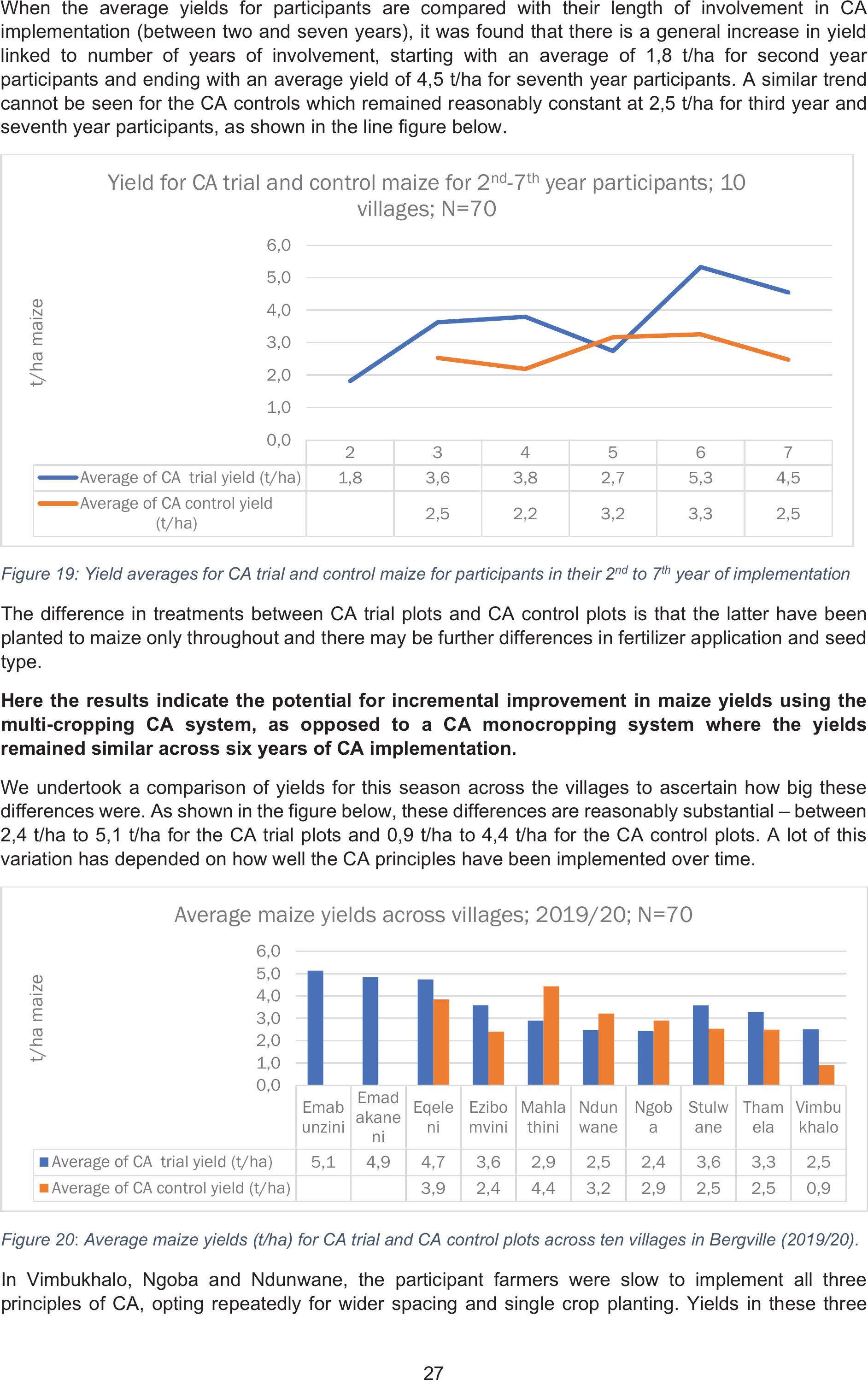
27
When the average yields for participants are compared with their length of involvement in CA
implementation (between two and seven years), it was found that there is a general increase in yield
linked to number of years of involvement, starting with an average of 1,8 t/ha for second year
participants and ending with an average yield of 4,5 t/ha for seventh year participants. A similar trend
cannot be seen for the CA controls which remained reasonably constant at 2,5 t/ha for third year and
seventh year participants, as shown in the line figure below.
Figure 19: Yield averages for CA trial and control maize for participants in their 2nd to 7th year of implementation
The difference in treatments between CA trial plots and CA control plots is that the latter have been
planted to maize only throughout and there may be further differences in fertilizer application and seed
type.
Here the results indicate the potential for incremental improvement in maize yields using the
multi-cropping CA system, as opposed to a CA monocropping system where the yields
remained similar across six years of CA implementation.
We undertook a comparison of yields for this season across the villages to ascertain how big these
differences were. As shown in the figure below, these differences are reasonably substantial – between
2,4 t/ha to 5,1 t/ha for the CA trial plots and 0,9 t/ha to 4,4 t/ha for the CA control plots. A lot of this
variation has depended on how well the CA principles have been implemented over time.
Figure 20: Average maize yields (t/ha) for CA trial and CA control plots across ten villages in Bergville (2019/20).
In Vimbukhalo, Ngoba and Ndunwane, the participant farmers were slow to implement all three
principles of CA, opting repeatedly for wider spacing and single crop planting. Yields in these three
234567
Average of CA trial yield (t/ha)1,8 3,6 3,8 2,7 5,3 4,5
Average of CA control yield
(t/ha) 2,5 2,2 3,2 3,3 2,5
0,0
1,0
2,0
3,0
4,0
5,0
6,0
t/ha maize
Yield for CA trial and control maize for 2nd-7th year participants; 10
villages; N=70
Emab
unzini
Emad
akane
ni
Eqele
ni
Ezibo
mvini
Mahla
thini
Ndun
wane
Ngob
a
Stulw
ane
Tham
ela
Vimbu
khalo
Average of CA trial yield (t/ha)5,1 4,9 4,7 3,6 2,9 2,5 2,4 3,6 3,3 2,5
Average of CA control yield (t/ha)3,9 2,4 4,4 3,2 2,9 2,5 2,5 0,9
0,0
1,0
2,0
3,0
4,0
5,0
6,0
t/ha maize
Average maize yields across villages; 2019/20; N=70

28
villages averaged 2,5 t/ha this season. Eqeleni, Ezibomvini and Stulwane are the three villages where
participants have most consistently employed multiple cropping options and rotations in their six years
of involvement and yields for these three villages averaged around 4 t/ha this season.
For the villages involved for three to four years in CA implementation, a similar trend can be seen. For
the two villages where participants did not consistently undertake multiple cropping and crop rotation
options (Thamela and Mahlathini), the average yield is around 3,1 t/ha and for the two villages where
these options were included (Emabunzini and Emadakaneni), the average yield this season was 5 t/ha.
In conclusion, there is no linear relationship between yield and length of involvement in CA
implementation, but there is a definite trend of improved yields for those participants who more
consistently included the multiple cropping options in their CA trials.
2
2.2.4
Bulk density
Soil bulk density (ȡE), also known as dry bulk density, is the weight of dry soil (mass of solids) divided
by the total soil volume (Vsoil). Total soil volume is the combined volume of solids and pores which may
contain air (Vair) or water (Vwater), or both.
High bulk density is an indicator of low soil porosity and soil compaction, which may cause restrictions
to root growth, and poor movement of air and water through the soil. It has also been shown that
minimum tillage practices increase bulk density without restricting aeration and water movement in the
soil, compared to the same soils under tillage (Cavalieri, da Silva, Leão, Dexter, & Håkansson, 2009).
In general, bulk densities greater than 1,6 g/cm3tend to restrict root growth (McKenzie, Jacquier, Isbell,
& and Brown, 2004). Sandy soils usually have higher bulk densities (1,3-1,7 g/cm3) than fine silts and
clays (1,1-1,6 g/cm3) because they have larger, but fewer pore spaces. In clay soils with good soil
structure, there is more pore space because the particles are very small, and many small pore spaces
fit between them. Soils rich in organic matter (e.g. peaty soils) can have densities of less than 0,5 g/cm3.
On cropland, long-term solutions to bulk density and soil compaction problems revolve around
decreasing soil disturbance and increasing soil organic matter. A system that uses cover crops, crop
residues and/or reduced tillage results in increased soil organic matter, less disturbance and reduced
bulk density. Additionally, the use of multi-crop systems involving plants with different rooting depths
can help break up compacted soil layers.
The small table below outlines the relationship between soil type and bulk density (NRCS, 2011).
General relationship of soil bulk density to root growth based on soil texture
Soil Texture Ideal bulk densities for plant
growth (g/cm3)
Bulk densities that restrict root
growth (g/cm3)
Sandy <60 >1,80
Silty <1,40 >1,65
Clayey <1,10>1,47
Samples were collected from the top 5 cm of soil using sampling rings 7,2 cm in diameter using the
following procedure:
xThe ring was pushed (buried) into the ground using a piece of wood and a hammer (the
piece of wood was used to protect the ring).
xA spade was used to dig the ring out of the soil.
xExcess soil sticking out of the ring was cut using a knife to ensure the soil fitted perfectly
into the ring (making sure the volume was the same for all samples).
xThe soil samples (in the ring) were wrapped with aluminium foil and transported to the lab
for analysis.
xAt the lab, samples were unwrapped, placed in aluminium dishes, weighed and assigned
codes, and put in an oven to dry at 100°C for 48 hours.

29
xAfter 48 hours, samples were weighed and the masses were recorded for calculation of dry
mass.
Figure 21: Left to right: Sampling procedure for bulk density
The equation used to calculate the total soil volume is shown below.
ܸ݈ݑ݉݁(௦) =ߨݎଶ×݀
Where, ʌ is pi, r is radius and d is depth for the ring, volume was calculated in cm3 and mass of the
sample was measured in grams (g).
Average dry mass for all samples collected in the same plot was used to calculate the bulk density and
the same volume (based on the dimensions of the ring) was used. Equation 2 was used to calculate
the ȡE
ܤݑ݈݇݀݁݊ݏ݅ݐݕ(ܤܦ)=ܯܽݏݏ݂ݏ݈݅(݃)
ܸ݈ݑ݂݉݁ݏ݈݅(ܿ݉ଷ)
Below is a summary of the results of bulk density calculations for different cropping practices within the
CA system for three participants in Bergville. They were chosen for having differing periods of cropping
under CA and for inclusion of several practices within their CA system – intercropping and planting of
summer cover crops (SCC).
Table 8: Bulk density (pb) results for three CA participants (2019)
Village
Period unde
r
CA (yrs)
Name and
surname
Control CT
Control CA
M
M+B
M+CP
SCC
Average
Ezibomvini5 Phumelele Hlongwane1,30 1,36 1,38 1,33 1,38 1,28 1,34
Eqeleni 6 NtombakheZikode 1,35 1,49 1,37 1,32 1,38
Thamela 2 Mkhuliseni Zwane1,14 1,08 1,09 1,07 1,10
Average bulk density 1,27
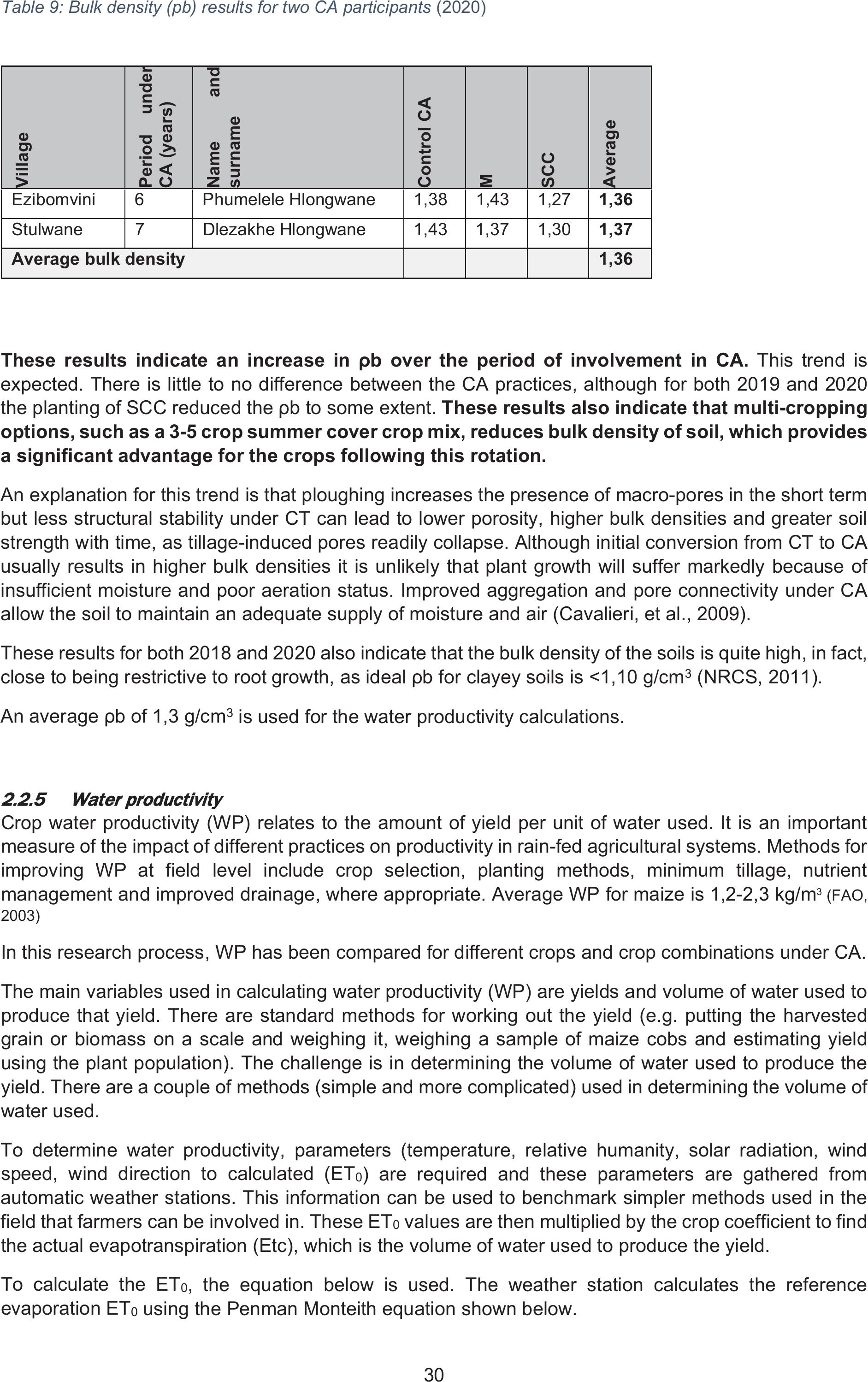
30
Table 9: Bulk density (pb) results for two CA participants (2020)
7KHVH UHVXOWV LQGLFDWH DQ LQFUHDVH LQ ȡE RYHU WKH SHULRG RI LQYROYHPHQW LQ &$ This trend is
expected. There is little to no difference between the CA practices, although for both 2019 and 2020
WKHSODQWLQJRI6&&UHGXFHGWKHȡEto some extent. These results also indicate that multi-cropping
options, such as a 3-5 crop summer cover crop mix, reduces bulk density of soil, which provides
a significant advantage for the crops following this rotation.
An explanation for this trend is that ploughing increases the presence of macro-pores in the short term
but less structural stability under CT can lead to lower porosity, higher bulk densities and greater soil
strength with time, as tillage-induced pores readily collapse. Although initial conversion from CT to CA
usually results in higher bulk densities it is unlikely that plant growth will suffer markedly because of
insufficient moisture and poor aeration status. Improved aggregation and pore connectivity under CA
allow the soil to maintain an adequate supply of moisture and air (Cavalieri, et al., 2009).
These results for both 2018 and 2020 also indicate that the bulk density of the soils is quite high, in fact,
close to being restrictive to root growth, as ideal ȡEIRUFOD\H\VRLOVLVJFP3 (NRCS, 2011).
An DYHUDJHȡERI g/cm3 is used for the water productivity calculations.
2
2.2.5
Water productivity
Crop water productivity (WP) relates to the amount of yield per unit of water used. It is an important
measure of the impact of different practices on productivity in rain-fed agricultural systems. Methods for
improving WP at field level include crop selection, planting methods, minimum tillage, nutrient
management and improved drainage, where appropriate. Average WP for maize is 1,2-2,3 kg/m3 (FAO,
2003)
In this research process, WP has been compared for different crops and crop combinations under CA.
The main variables used in calculating water productivity (WP) are yields and volume of water used to
produce that yield. There are standard methods for working out the yield (e.g. putting the harvested
grain or biomass on a scale and weighing it, weighing a sample of maize cobs and estimating yield
using the plant population). The challenge is in determining the volume of water used to produce the
yield. There are a couple of methods (simple and more complicated) used in determining the volume of
water used.
To determine water productivity, parameters (temperature, relative humanity, solar radiation, wind
speed, wind direction to calculated (ET0) are required and these parameters are gathered from
automatic weather stations. This information can be used to benchmark simpler methods used in the
field that farmers can be involved in. These ET0 values are then multiplied by the crop coefficient to find
the actual evapotranspiration (Etc), which is the volume of water used to produce the yield.
To calculate the ET0, the equation below is used. The weather station calculates the reference
evaporation ET0using the Penman Monteith equation shown below.
Village
Period unde
r
CA (years)
Name and
surname
Control CA
M
SCC
Average
Ezibomvini6 Phumelele Hlongwane 1,38 1,43 1,27 1,36
Stulwane 7 Dlezakhe Hlongwane1,43 1,37 1,301,37
Average bulk density 1,36

31
ܧܶ=
0.408ο(ܴെܩ
)+ߛ900
ܶ+273 ݑଶ(݁௦െ݁
)
ο+ߛ(1 + 0.34ݑଶ)
Where,
ET0 is reference evapotranspiration (mm/day)
Rn is net radiation at the crop surface (MJ m-2 day-1)
G is soil heat flux density (MJ m-2 day-1)
T is air temperature at 2 m height (°C)
u2 is wind speed at 2 m height (m s-1)
es is saturation vapour pressure (kPa)
D is slope vapour pressure curve (kPa °C-1)
g is psychrometric constant (kPa °C-1).
Water productivity was calculated for two participants in Bergville (2019), Phumelele Hlongwane
(Ezibomvini) and Ntombakhe Zikode (Eqeleni). Both participants had been implementing CA for a
period of five years. Water productivity for different CA cropping options was calculated for both
participants; in this case using the grain weight only.
The options were a M-CA control (consecutively mono-cropped maize); M-CA trial (single cropped
maize in a rotation system); M+C-CA trial (maize and cowpea intercropped plot in a rotation system)
and CA-M+B trial (maize and bean intercropped plot in a rotation system). The aim was to ascertain
whether the different cropping options within the CA system provide for different water productivity
outcomes. The results are shown in the figure below.
Figure 22: Water productivity for different CA cropping options for 2 participants (2019)
M-CA
trial
M _CA
Control
M+C-
CA Trial
M + B-
CA Trial
M-CA
Control
M + B-
CA Trial
M + B-
CA Trial
M+C-
CA Trial
PH PH PH PH NZNZNZNZ
WP (kg/m3)2,18 3,53 3,17 4,40 1,04 1,15 1,33 0,86
0,00
0,50
1,00
1,50
2,00
2,50
3,00
3,50
4,00
4,50
5,00
Water Productivty (kg/m3)
WP (kg/m3)PH - PhumeleleHlongwane
NZ - Ntombakhe Zikode
(g )
,
,
,
,
,
,
,
(g )
,
,
,
,
,
,
,
M=Maize B=Beans C=Cowpeas

32
A similar process was undertaken for 2020, but in this case WP calculations were done for four
participants across four villages, to expand the exploration.
Figure 23: Water productivity for different CA cropping options for 4 participants (2020)
Comparing Figures 20 and 21, the following trends can be seen:
xWater productivity for both Phumelele Hlongwane and Ntombakhe Zikode are lower for the
2020 season than in 2019.
xIn both seasons, Phumelele Hlongwane’s water productivity, for all the crop combinations
tested, are higher than that of the other participants.
xFor both seasons, intercropped CA plots (both M+B and M+CP) are higher than single
cropped CA-M plots.
xWater productivity for conventionally tilled maize is lower than the CA control maize plot.
Water productivity for CA maize grown as an intercrop with beans or cowpeas is higher than
single cropped CA maize and water productivity for CA plots is higher than conventionally tilled
plots. Despite annual differences in water productivity, these trends remained the same across
two seasons.
The CWP was also calculated
for the above-ground maize
plant material (stalks and
leaves). Again, there is a very
clear trend of much improved
WP for the maize when
intercropped with either beans or
cowpeas. The small figure
alongside provides an average
for Bergville (four participants
across four villages) for the
2019/20 cropping season.
CA-
M+B CA-M
CA:M
-
Contr
CA-M CA-
M+B CA-M Contr
-M CA-M
CA-
M+C
P
CA-M CA-M
Conv.
Contr
-M
CA-M CA-
M+B
CA-
M+B CA-M CA-
M+B
CA:M
-
Contr
CA-
M+B
CA:M
-
Contr
CA-
M+C
P
NZNZNZNZNZNMNMNMNMNMNMPH PH PH PH PH PH PH BH BH BH
EqeEqeEqeEqeEqeStuStuStuStuStuStuEzi Ezi Ezi Ezi Ezi Ezi EziNduNduNdu
BERGVILLE
Water Productivity (kg/m3)1,55 1,03 0,75 0,86 1,54 0,71 1,56 1,21 1,99 1,40 0,85 0,58 1,16 2,37 1,93 1,67 2,38 1,16 1,11 1,10 2,19
0,00
0,50
1,00
1,50
2,00
2,50
Water Productivty (kg/m3)
WP (kg/m3)PH - Phumelele
Hlongwane
NZ - Ntombakhe
Zikode
NM -Nelisiwe
Msele
BH - Boniwe
Hlatshwayo
M=Maize
B=Beans
C=Cowpeas
0
,
0,
W
0
0,5
W
0
0,5
W
Eqe=Eqeleni
Stu=Stulwane
Ezi=Ezibovini
Ndu=Ndunwane
CA:M-
Contr CA-MCA-M+B CA-M+CPConv.
Contr-M
Total 6,297,0613,66 12,473,17
0,00
5,00
10,00
15,00
kg/m3
Maize biomass CWP

33
2
2.2.6
Examples of farmer-level experimentation in Bergville
The photographs below provide a visual snapshot of some of the farmer-level experiments undertaken.
Figure 24: Stuwlane; Left: Chupile Buthelezi’s maize and scc (sunflower, Sun hemp and millet) intercrop. Centre:
Khulekani Dladla’s maize and bean intercrop and a plot of sunflowers. Right: Nelisiwe Msele’s CA trial with SCC
in the foreground.
Figure 25: Ezibomvini: Left: Nombono Dladla’s CA trial with Dolichos (LL) and a maize and cowpea intercropped
plot in the foreground. Centre: Phumelele Hlongwane’s maize and bean intercropped CA plot. Right: Velephi
Zimba standing in her SCC plot (Sun hemp, millet and sunflower).
Figure 26: Eqeleni: Left: Ntbombakhe Zikode’s WCC Isaia oats, fodder rye, fodder radish) CA trial plot. Centre:
Smephi Hlatshwayo’s single cropped CA maize. Right: Thulile Zikode’s SCC (millet, Sun hemp and sunflower)
CA plot.

34
2.3 LIVESTOCK INTEGRATION
Livestock are an important component of the smallholder farming system and crop-livestock integration
can offer important gains in terms of sustainability and climate resilience.
Aspects of crop-livestock integration that were considered are the following:
xInclusion of fodder species for poultry and livestock into the cover crop mixes in the rotation
and multi-cropping system, including summer (sunflower, millet, Sun hemp, Dolichos
beans, cowpeas) and winter (Saia oats, fodder rye, fodder radish) cover cropping options.
xWinter fodder supplementation.
xStrip cropping with perennial fodder species.
2
2.3.1
Cover crop mixes
The summer cover crops (millet, Sun hemp, sunflower, sorghum) have been planted either in separate
blocks or as intercropping options with maize. Some participants practiced a cut and carry system for
their livestock, but mostly these crops are left to seed and the seed used as feed for poultry. Winter
cover crops have been grazed directly off the fields when cattle are let in, usually towards the end of
May.
Figure 27: Examples of cover crop seeds kept by participating farmers. Left: sorghum. Centre: Sun hemp and
forage sorghum. Right: Babala (millet).
Despite the advantages in soil health, yields and fodder availability that these experiments have shown,
farmers have been slow to expand the areas under cover crop production due to a combination both of
difficulty in paying for seed and a conception that
due to limited field sizes and labour, a focus
entirely on food production for themselves is the
only option.
2.3.2
Winter foddersupplementation
experimentation
Participants undertook to provide
supplementation for a selection of their livestock
which required supplementation, mainly cows
with calves or sick and ailing animals. A body
condition score sheet (shown right) was used to
assess the outcome of the supplementation,
which was continued for a minimum of one
month.
A process was undertaken to cut and bale veld
grass as well as a proportion of the cover crop

35
residues participants had planted – namely cowpea, Dolichos bean, teff and maize. In addition,
supplements were introduced that could be included in these “rations” for winter feeding. These included
LS 33 and Premix 450. Seven participants undertook this experimentation process and five of these
participants recorded their feeding as well as the results using the livestock condition scoring sheet, as
shown in the table below.
Table 10: Fodder supplementation experimentation (2018/19)
VillageName and
surname
BalesSupplementsFeeding regime
(with start date)
Condition
scoring
EzibomviniPhumelele
Hlongwane
32 – veld grassLS33 (12 L),
premix 450 (2x50
kg)
2 cows – 1x/day (1
September)
From 2 to 4
StulwaneMtholeni
Buthelezi
40 – veld grassLS33 (8,8 L),
premix (50 kg)
4 of 16 cows – every
2nd day (12 August)
From 2 to 4
Thulani Dlamini9 – Lab-lab
3 – grass, maize stalks,
cowpea
LS33 (4,8 L)5 of 17 – every 2nd
day (1 September)
From 2 to 3
Dlezakhe
Hlongwane
10 – veld grass, Lablab,
cowpeas, maize stalks
LS33 (4 L), premix
450 (50 kg)
4 of 19 – every 2nd
day (1 September)
From 0 to 3
EqeleniNtombakhe
Zikode
6 – veld grass
2 – teff
LS33 (4 L), premix
450 (50 kg)
1 of 4 – every 2nd
day
(1 September)
From 2 to 4
In general, this process managed to either maintain or improve the livestock’s condition for all seven
participants. At the end of the experimental process, livestock were all scored at ratings 3 (ribs well
covered and body outline smooth) or 4 (ribs not visible and body outline rounded), according to the
condition scoring sheet shown above.
Participants were very satisfied with the outcomes of these experiments and felt that they could continue
with supplementation in future. The supplements are relatively cheap and now that they have some
experience with cutting and baling grass, they also feel this is manageable and a good idea.
Participants also commented that they did not need to herd the animals that were being fed as they all
started coming home to the kraal in the evenings for their “meals”. This is a major advantage.
Participants also agreed that the cattle prefer the LS33 over the premix 450. The LS33 however, is a
bit more expensive (R180/20 L versus R230/50 kg). Sixteen participants (50% were women)
volunteered to try out the supplementation experimentation process in the coming season. In addition,
a brush cutter was procured for the learning groups to facilitate the cutting and baling of grass.
Figure 28: Left: A manual baler (background) being used to make veld grass bales (foreground). Centre:
Phumelele Hlongwane measuring out the daily Premix 450 ration for her cows. Right: Khulekani Dladla’s bales
stored in an unused rondavel for later use.
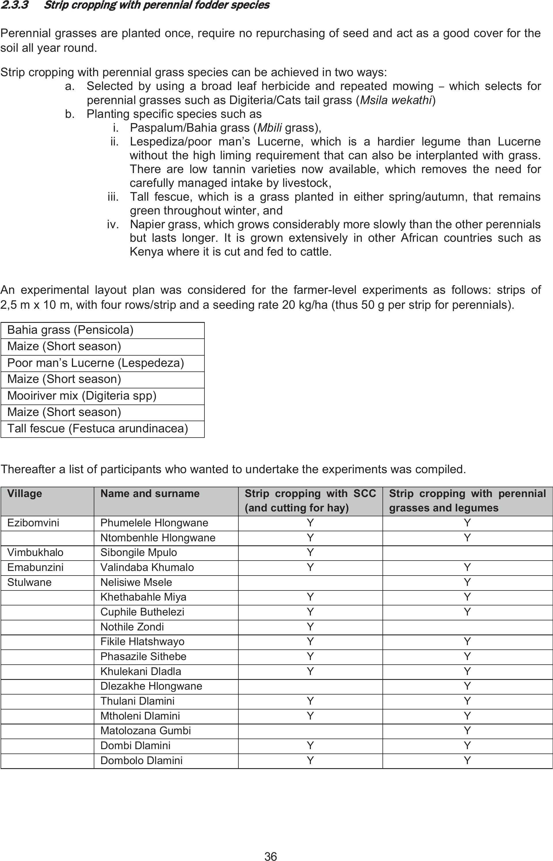
36
2
2.3.3
Strip cropping with perennial fodder species
Perennial grasses are planted once, require no repurchasing of seed and act as a good cover for the
soil all year round.
Strip cropping with perennial grass species can be achieved in two ways:
a. Selected by using a broad leaf herbicide and repeated mowing – which selects for
perennial grasses such as Digiteria/Cats tail grass (Msila wekathi)
b. Planting specific species such as
i. Paspalum/Bahia grass (Mbili grass),
ii. Lespediza/poor man’s Lucerne, which is a hardier legume than Lucerne
without the high liming requirement that can also be interplanted with grass.
There are low tannin varieties now available, which removes the need for
carefully managed intake by livestock,
iii. Tall fescue, which is a grass planted in either spring/autumn, that remains
green throughout winter, and
iv. Napier grass, which grows considerably more slowly than the other perennials
but lasts longer. It is grown extensively in other African countries such as
Kenya where it is cut and fed to cattle.
An experimental layout plan was considered for the farmer-level experiments as follows: strips of
2,5 m x 10 m, with four rows/strip and a seeding rate 20 kg/ha (thus 50 g per strip for perennials).
Bahia grass (Pensicola)
Maize (Short season)
Poor man’s Lucerne (Lespedeza)
Maize (Short season)
Mooiriver mix (Digiteria spp)
Maize (Short season)
Tall fescue (Festuca arundinacea)
Thereafter a list of participants who wanted to undertake the experiments was compiled.
Village Name and surname Strip cropping with SCC
(and cutting for hay)
Strip cropping with perennial
grasses and legumes
Ezibomvini Phumelele HlongwaneY Y
Ntombenhle HlongwaneY Y
Vimbukhalo Sibongile Mpulo Y
Emabunzini Valindaba Khumalo Y Y
Stulwane Nelisiwe MseleY
Khethabahle Miya Y Y
Cuphile Buthelezi Y Y
Nothile Zondi Y
Fikile Hlatshwayo Y Y
Phasazile SithebeY Y
Khulekani Dladla Y Y
Dlezakhe Hlongwane Y
Thulani Dlamini Y Y
Mtholeni DlaminiY Y
Matolozana GumbiY
Dombi Dlamini Y Y
Dombolo Dlamini Y Y

37
Strip cropping trials were initiated in the middle of January 2020. Ten of the 15 volunteers planted their
strip cropping trials. Germination of the grass species was, however, extremely patchy and quite low in
most cases. Some of the plots were overrun by weeds, at which point neither the farmers nor the
facilitators could identify the grass species from the weed species.
Figure 29: Left: Nothile Zondi’s strip cropping trial with the short season maize strips growing vigorously and the
Lespedeza strip showing some growth. Right: The Mooiriver mix (Digiteria) did not germinate.
Figure 30: Right: An overgrowth of weeds in
Thulani Dlamini’s strip cropping trial plot made
identification of the planted grass species virtually
impossible
Khulekani Dladla tried to deal with the hot dry
conditions in his strip cropping trial plot by
mulching, which helped, and he managed to
get the Lespedeza and Pensacola (Tall
Fescue) to grow.
Figure 31: Left: Kulekhani Dladla mulched his strip cropping trail. Right: Germination and initial growth for
Pensacola (Bahia grass) was promising, upon monitoring in early March 2020.
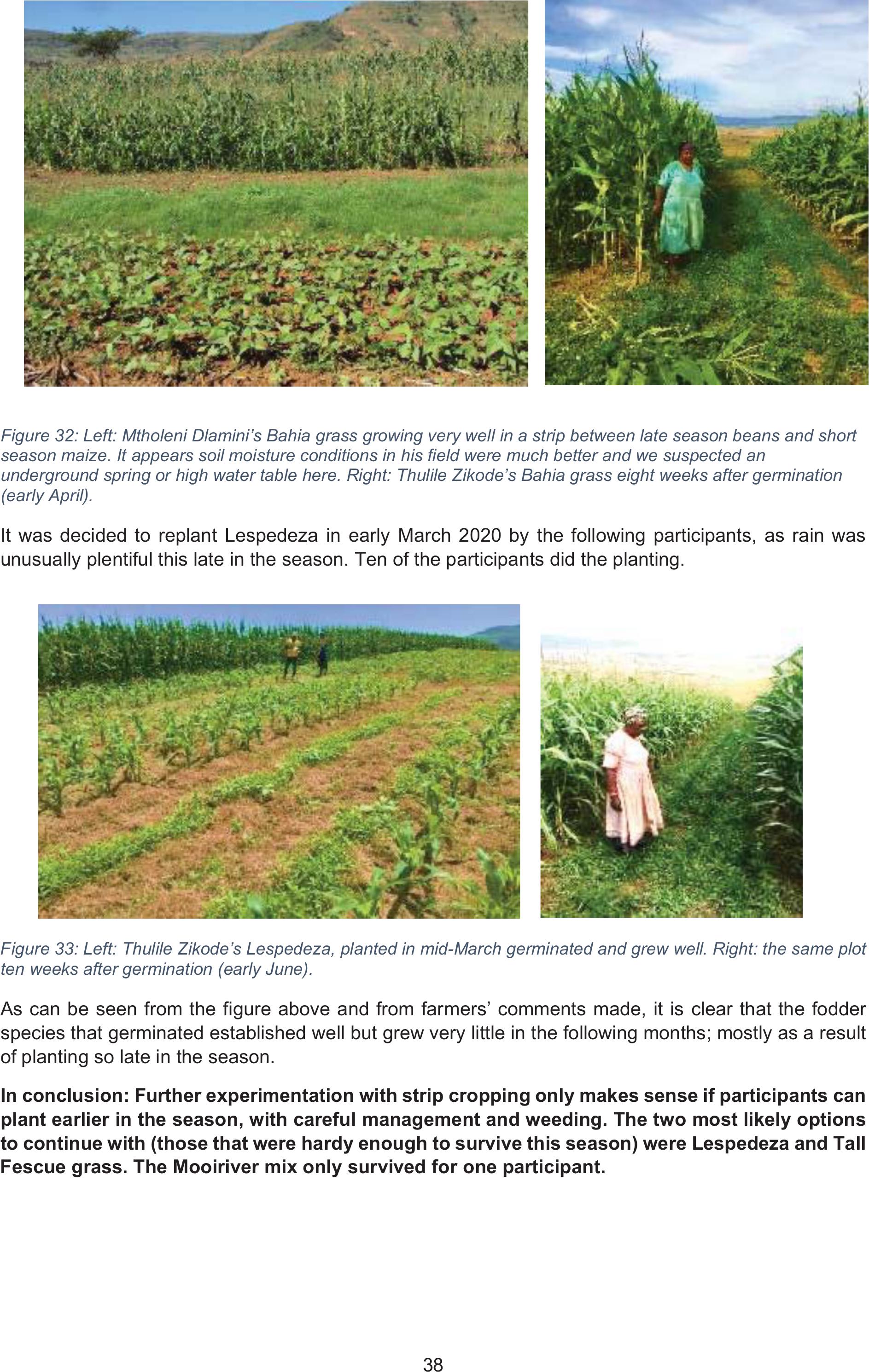
38
Figure 32: Left: Mtholeni Dlamini’s Bahia grass growing very well in a strip between late season beans and short
season maize. It appears soil moisture conditions in his field were much better and we suspected an
underground spring or high water table here. Right: Thulile Zikode’s Bahia grass eight weeks after germination
(early April).
It was decided to replant Lespedeza in early March 2020 by the following participants, as rain was
unusually plentiful this late in the season. Ten of the participants did the planting.
Figure 33: Left: Thulile Zikode’s Lespedeza, planted in mid-March germinated and grew well. Right: the same plot
ten weeks after germination (early June).
As can be seen from the figure above and from farmers’ comments made, it is clear that the fodder
species that germinated established well but grew very little in the following months; mostly as a result
of planting so late in the season.
In conclusion: Further experimentation with strip cropping only makes sense if participants can
plant earlier in the season, with careful management and weeding. The two most likely options
to continue with (those that were hardy enough to survive this season) were Lespedeza and Tall
Fescue grass. The Mooiriver mix only survived for one participant.

39
3 BEST PRACTISE OPTIONS IN LEARNING METHODOLOGY
3.1 LEARNING METHODOLOGY
The CA experimentation workshops are run over a period of two to three days, starting with a day of
theory and discussion followed by practical demonstrations, after which the farmer volunteers plant their
own trial and control plots.
Minimum tillage and soil cover are not intuitive concepts for smallholders, as these directly oppose their
normal or habitual farming practices. The presentation of the CA principles and reasoning is done with
as many photographs and visual examples as possible; either using a PowerPoint presentation or using
A4 colour plates as visuals. Topics covered in the
presentation include principles of CA, different planting
options and planters, farmer-level experimentation and layout
of CA trials, intercropping examples, reduction in runoff,
cover crop options (summer and winter combinations and a
farmer case study).
Figure 34: Introduction of concepts in CA and cover crops using printed slides in two different villages
Comments from the Limpopo groups included:
x“Use of pictures in the slides helped us to visualise what was being taught.”
x“Maybe you should make notes on the flipchart in Sepedi and not English to allow us to also
take notes.”
x“You keep showing us examples of CA from other places, is it because you do not have local
examples?”
x“One thing that is clear is that we have not left as much soil cover as we see in the pictures.
This could be because in winter we clear and turn the field cropping plots into a garden. This
also means that we till the soil, so we haven’t minimised the tilling. This has led to a lot of runoff
in the plots and in summer the rain washes away the seed and causes erosion.”
x“Seeing examples of places where CA has worked gives us courage to keep trying. One day
we might realise the same benefits. Even with the high level of uncertainty it is worth trying.”
x“It seems in the examples shown on the slides, the people have access to water or it rains a lot
in their area.”
These comments have assisted the team to fine-tune the learning process to be as participatory and
locally appropriate as possible.
3.2 PRACTICAL DEMONSTRATIONS
For the practical demonstrations, a template using knotted ropes and pegs is used to assist farmers to
understand and internalise the layout and the importance of close spacing. The concept of staggered
or zigzag planting is also demonstrated. The spacing is designed to ensure the development of an early
canopy cover for weed control, while minimising competition between plants.

40
Figure 35: Left: A demonstration plot in Bergville, working with the rope templates for planting. Right: Mpelesi
Sekgobela from Sedawa planting using the template.
In Limpopo, we also worked with participants to draw the layout on flip chart paper, for them to keep as
a record and reminder. This practice worked quite well here, but not in KZN, where literacy levels in the
learning groups was generally lower.
Figure 36: Left: Mr S Selala, the facilitator, showing the layout drawing/template in Turkey. Centre: Using a
variation with the actual seed laid out on the paper. Right: Abitha Shaai in Willows drawing out her learning
group’s layout template.
For the demonstrations and farmer-led trials, participants were supported with provision of seed,
planters and other inputs as agreed upon. This was to reduce the risk in trying out new and unfamiliar
practices. The control plots were managed by participants in their normal way.
Farmer comments regarding the learning demonstrations:
x“This is the easiest way to plant. If I had used this method from the beginning, I would have
finished planting the whole yard in less than two days.”
x“This CA method requires less labour and also less seed than our normal way of planting.”
x“We are not used to leaving residues on the soil surface; we usually remove weeds and organic
matter and then burn it. We see now that maybe residue is important, but it is difficult, as we
are used to seeing nice clean plots and this looks very messy. It is going to take us a while to
get used to this.”

41
x“We would need to make some adjustments in the way we do our cropping; dividing our fields
into two parts (garden area) and (field cropping area) and minimising or stopping burning of dry
weeds and crop residues, even though this is tricky as the crop residues take some time to
break down in the soil and snakes can hide in this mulch and make it unsafe for children to play
there.”
x“The spacing, especially between the beans, really seems to be too narrow. We are sure there
will be competition.”
x“We appreciated that you are patient with us, it helps us when our memories are being
refreshed; even though we should know this very well by now.”
x“You always try new methods to help us understand the subject matter.”
x“Please provide us with some sort of a template on how to plant different combinations under
CA, something that will look like a calendar that I can paste on a wall.”
x“We don’t collect wood anymore as such and ropes are not really available in the households,
but we will share the existing rope templates and try our best.”
x“Making the template was easy and it made the job a lot easier.”
x“Overall, we loved the layout made with seed on paper, I don’t think I can forget this.”
x“It is a good idea to work together to plant these trials. That way we can remind each other and
also plant faster.”
3
3.2.1
No-till planters
No-till planters are an important aspect of implementation of a CA cropping system. These are provided
to the learning groups to share and use. As farmers become more familiar with the process, they are
encouraged to purchase their own planters, either as individuals or as groups.
Different planters have been introduced:
xHand-held planters (MBLI planters and Haraka planter).
xAnimal-drawn planters (modified Magoye rippers and Knapick planters).
xTractor-drawn planters (Eden Equip two-row planter).
Some illustrative photographs are shown below.
Figure 37: Left: Using MBLI planters. They operate similarly to hand hoes and are thus intuitive to use. Left:
Using a Haraka wheel planter. This planter only works with seed (and not fertilizer) but is much easier to use on
larger fields than the MBLI planters. Right: Three pictures illustrating use of a two-row tractor-drawn CA planter.

42
Figure 38:Left: Using a modified Magoye ripper no-till planter with oxen in KZN. Right: Testing the Knapick
planter with donkeys in Limpopo.
3
3.2.2
Facilitators’ reflections on the CA learning process
xThe concept of CA is knowledge intensive and difficult to convey in one learning session,
especially linked to deeply entrenched habits that work in opposition to the principles, such as
clearing and burning of weeds, wide spacing and the like.
xIt would be ideal to be able to run workshops through the whole cropping season to make
observations and deepen the learning.
xBecause the innovation system approach to learning relies on positive results from the farmer-
level experimentation, seasons such as the present one, where hot and dry conditions have
seriously hampered germination and growth, tend to be difficult for introduction of a new
practice. Farmers associate the lack of results with the practice, rather than the season. It can
be almost impossible to disentangle different factors, such as lack of soil fertility on the
performance of the trials as well. It is thus common to have very variable results within a group,
with some participants faring reasonably well and other failing completely. Under such
conditions, uptake of these practices tends to be low.
xParticipants somehow believe that this method cannot be used on larger fields as they have
now got into the habit of believing this is only possible with tractors and with assistance provided
in provision of seed. The concept of manual weeding is one they are not prepared to consider.
xThe habit of planting without any addition of soil nutrients or manure is a very common practice,
specifically in Limpopo, and is a big challenge when trying to improve yields. It is, however,
extremely difficult to persuade participants to collect and use manure. Many have no access
and would need to buy this from people who do, which is a constraint.

43
4 REFERENCES
Abawi, G.S. & Widmer, T.L. (2000). Impact of soil health management practices on soilborne
pathogens, nematodes and root diseases of vegetable crops.. Appl.Soil Ecol., Volume 15, pp. 37-47.
Bagyaraj, D.J. & Ashwin, R. (2017). Soil biodiversity: role in sustainable horticulture. Biodivers. Hortic.
Crops, Volume 5, pp. 1-18.
Cavalieri, K.M.V. et al. (2009). Long-term effects of no-tillage on soil physical properties in a Rhodic
Ferrasol in Paraná, Brzil. Soil and Tillage Research, Volume 103, pp. 158-164.
Critchley, W. & Siegert, K. (1991). Water harvesting (AGL/MISC/17/91). A Manual for the Design and
Construction of Water Harvesting Schemes for Plant Production. Rome: FAO.
Dlamini, P., Jewitt, G., Lorenz, S. & Orchard, C. (2011). Controlling factors of sheet erosion under
degraded grasslands in the sloping lands of KwaZulu-Natal, South Africa. Agricultural Water
Management, Volume 98 (11), pp. 1711-1718.
FAO (2003). Unlocking the Water Potential of Agriculture. [Online]
Available at: http://www.fao.org/3/y4525e/y4525e00.htm#Contents
FAO (2013). Climate Smart Agriculture Source Book. Rome,Italy: Food and Agriculture Organisation of
the United Nations.
Frac, M., Hannula, S.E., Belka, M.& Jedryczka, M. (2018). Fungal Biodiversity and Their Role in Soil
Health.. Front Microbiol.
Giller, K.E., Witter, E., Corbeels, M. & Tittonell, P. (2009). Review: Conservation agriculture and
smallholder farming in Africa; The heretic's view. Field Crops Research, pp. 23-34.
Goss, M.J. & deVarennes, A. (2002). Soil disturbance reduces the efficacy of mycorrhizal associations
for early soybean growth and N2 fixation. . 34, 1167-1173. doi:. Soil Biol. Biochem,Volume 34, pp.
1167-1173.
GRDC (2014). Measuring and monitoring changes in soil organic carbon accurately. s.l.:Department of
Agriculture and Food, Government of Western Australia.
Hoorman, J.J. (2020). CFAES. Role of soil bacteria. [Online]
Available at: https://ohioline.osu.edu/factsheet/anr-36
[Accessed 14 06 2020].
Ingham, E.R. (2009). Chapter 4: Soil Fungus . In: Soil Biology Primer. s.l.:Ankeny IA: Soil & Water
Conservation Society., pp. 22-23.
Johns, C. (2017). Living Soils: The Role of Microorganisms in Soil Health, Dalkeith, Australia: Future
Directions International. Strategic analysis paper.
Mchunu, C. & Chaplot, V. (2012). Land degradation impact on soil carbon losses through water erosion
and CO2 emissions. Geoderma, Volume 178, pp. 72-79.
Motaung, P. (2020). Evaluating soil health of smallholder maize monocrops and intercrops using
qualitative and quantitative soil quality assessment methods. Pretoria: MSc thesis in Soil Science,
University of Pretoria.
Mutema, M., Jewitt, G., Chivenge, P. & Kusangaya, S. (2017). Spatial scale impact on daily surface
water and sediment fluxes in Thukela river, South Africa..
Nel, W. (2009). Rainfall trends in the KwaZulu-Natal Dakensberg region of South Africa during the
twentieth century. Published online 12 December 2008 in Wiley InterScience (www.int. Int. J. Climatol.,
Volume 29, pp. 1634-1641.
Schulze, R.E. (2011). A 2011 Perspective on Climate Change and the South AfricanWater Sector.
Report TT 518/12.,Pretoria, RSA.: Water Research Commission.
Sheik, C.S. et al. (2011). Effect of warming and drought on grassland microbial communities. ISME J,
Volume 5 (10), pp. 1692-1700.

44
Smith, H., Kruger, E., Knot, J. & Blignaut, J. (2017). Chapter 12: Conservation Agriculture in South
Africa: Lessons from Case Studies. Conservation Agriculture for Africa: Building resilient farming
systems in a changing climate.. s.l.:CAB International.
Stolbovoy, V. et al. (2007). Soil sampling protocol to certify the changes of organic carbon stock in
minteral soil of the European Union. Version 2., Luxembourg. ISBN: 978-92-79-05379-5: EUR 21576
EN/2. 56 pp. Office for Official Publications of the European Communities.
Svenningsen, N.B. et al. (2018). Suppression of the activity of arbuscular mycorrhizal fungi by the soil
microbiota. THE ISME Journal,pp. 1296-1307.
Swanepoel, C.M., Swanepoel, L.H. & Smith, H.J. (2017). A review of conservation agriculture research
in South Africa. South African Journal of Plant and Soil, pp. 1-10.
Thierfelder, C. et al (2018). Complementary practices supporting conservation agriculture in Africa. A
review. Agronomy of Sustainable Development, Volume 38:16.
Veum, K.S., Lorenz, T. & Kremer, R.J. (2019). Phospholipid Fatty Acid Profiles of Soils under Variable
Handling and Sotrage Conditions. Agronomy Journal, 111(3), pp. 1091-1096.
Wikipedia (2020). Phospholipid-derived fatty acids. [Online]
Available at: "https://en.wikipedia.org/w/index.php?title=Phospholipid-
derived_fatty_acids&oldid=952758911"
